A Kalman filter incorporates uncertainty with inputs and observations to get better estimates of the sensor measurement. The purpose of this lab is to implement a Kalman Filter for ToF sensor readings. To perform the Drift Much Stunt in Lab 8, we need to turn before hitting the wall. As the sampling rate of the sensor in long distance mode is quite low, it is difficult to gauge where the robot is, especially when moving at a high speed. Using the Kalman Filter estimates will help estimate the distance from the wall when the sensor readings are not available.

Before starting this lab, I reviewed portions of lectures 11 and 12 which explain the implementation of a Kalman Filter.

Step Response

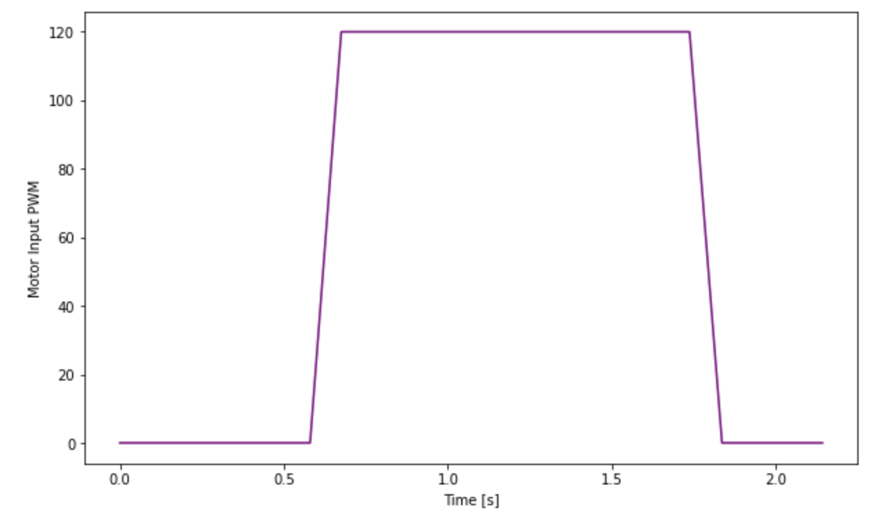
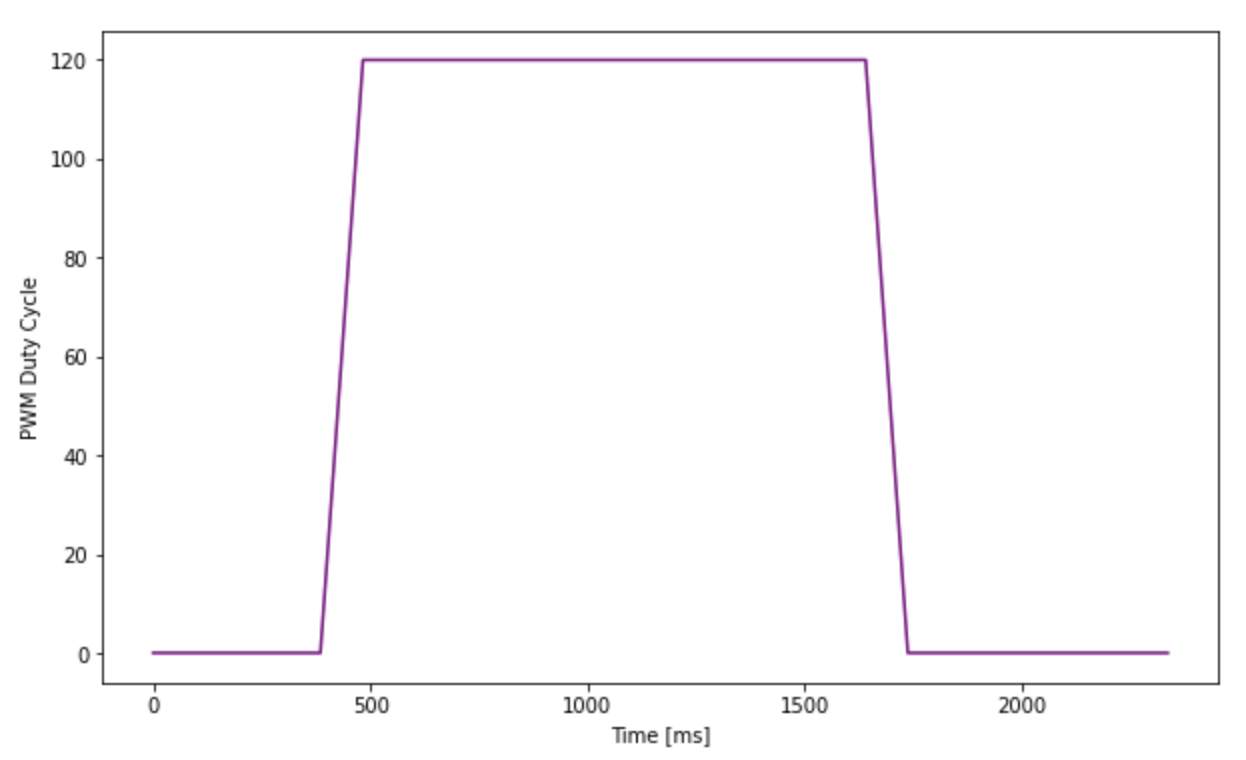
The State Space Equation used to in the Kalman Filter is dependent on drag and m. For a first order system, these terms can be calculated using the steady states speed and 90% rise time. To achieve steady state speed, I executed a step response by driving a car towards a wall with a PWM value of 120. This was the average PWM value (MIN_PWM = 90, MAX_PWM = 150) used in lab 6 while implementing PID control. The robot started off about 2m from the wall; Robot was stationary for the at least 600 msec, then a step size of 120 was given as motor input. As soon as the robot was less than 500 meters from the wall, the robot was stopped using active breaking.

The measurements from the ToF sensor (milli meters), running in Long Distance Mode with no timing budget set, were stored along with the time stamp and the motor input at that point. These stored values were sent to the computer after the run, via Bluetooth.

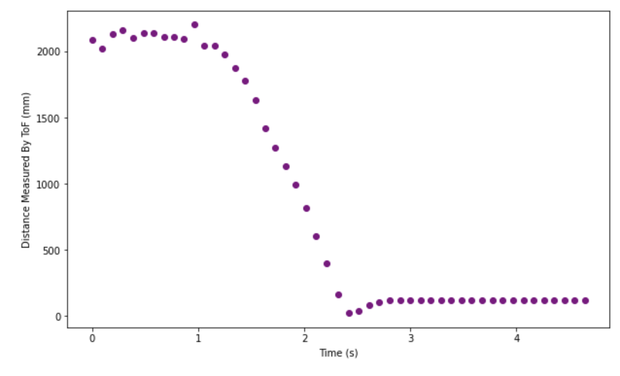
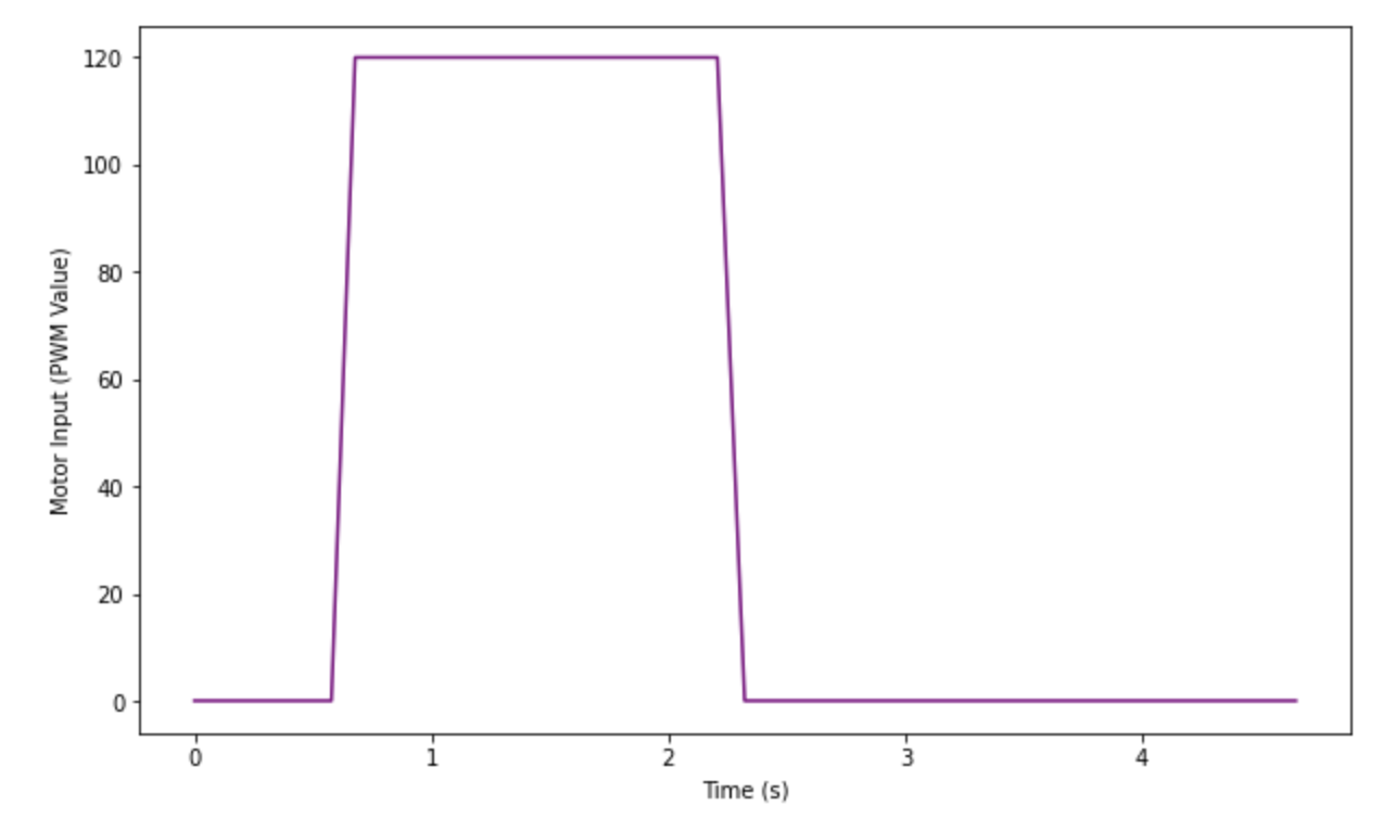
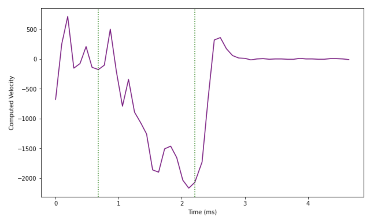
I used the np.gradient function with the distance and timestamps as parameters to generate the velocity graph. The calculated velocity is quite noisy; however, it does reach a steady state point towards the end. The two green lines in the graph represent the PWM value change. Note that before the step response is applied, the velocity is noisy, but it is more stable after the step response is removed. This might be because the sensor measurements are more accurate and stable when the wall is closer.

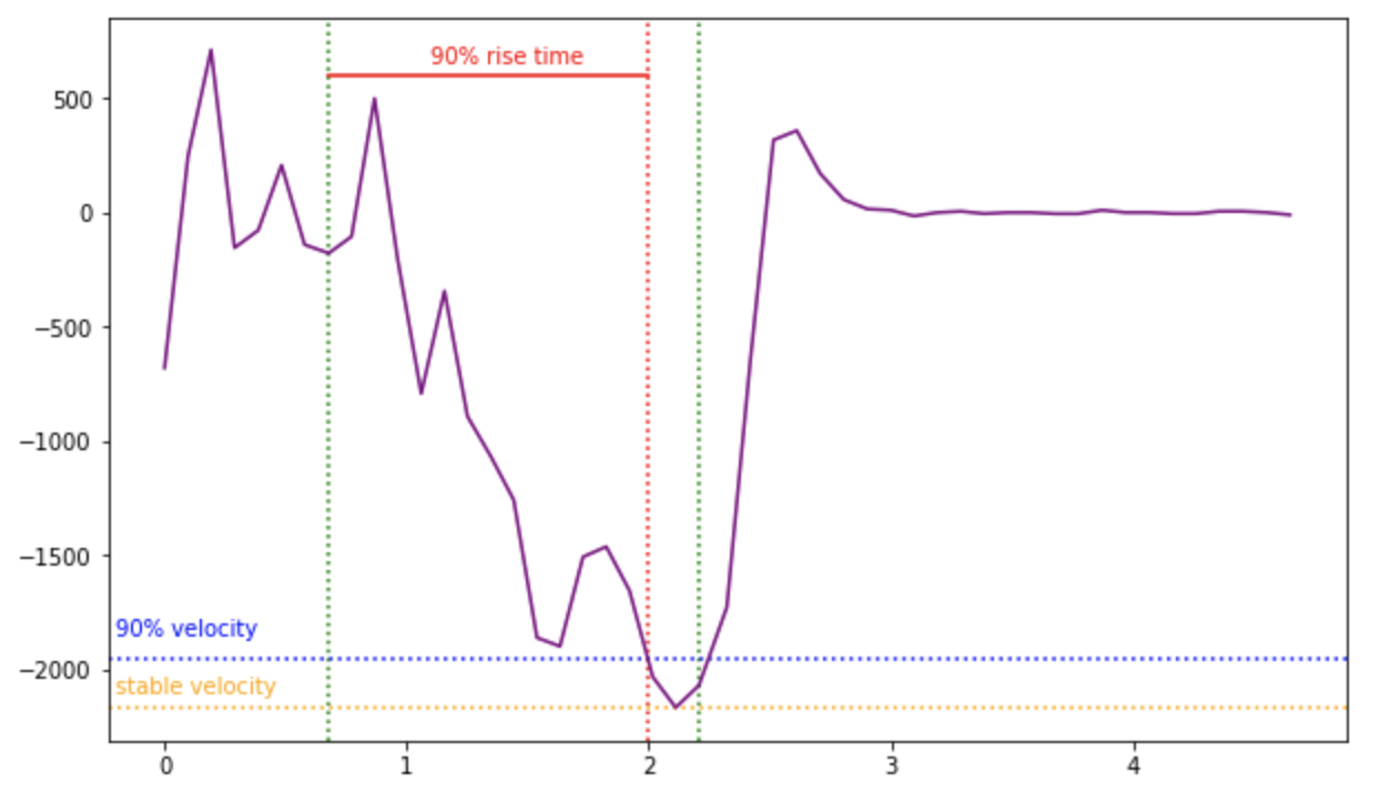
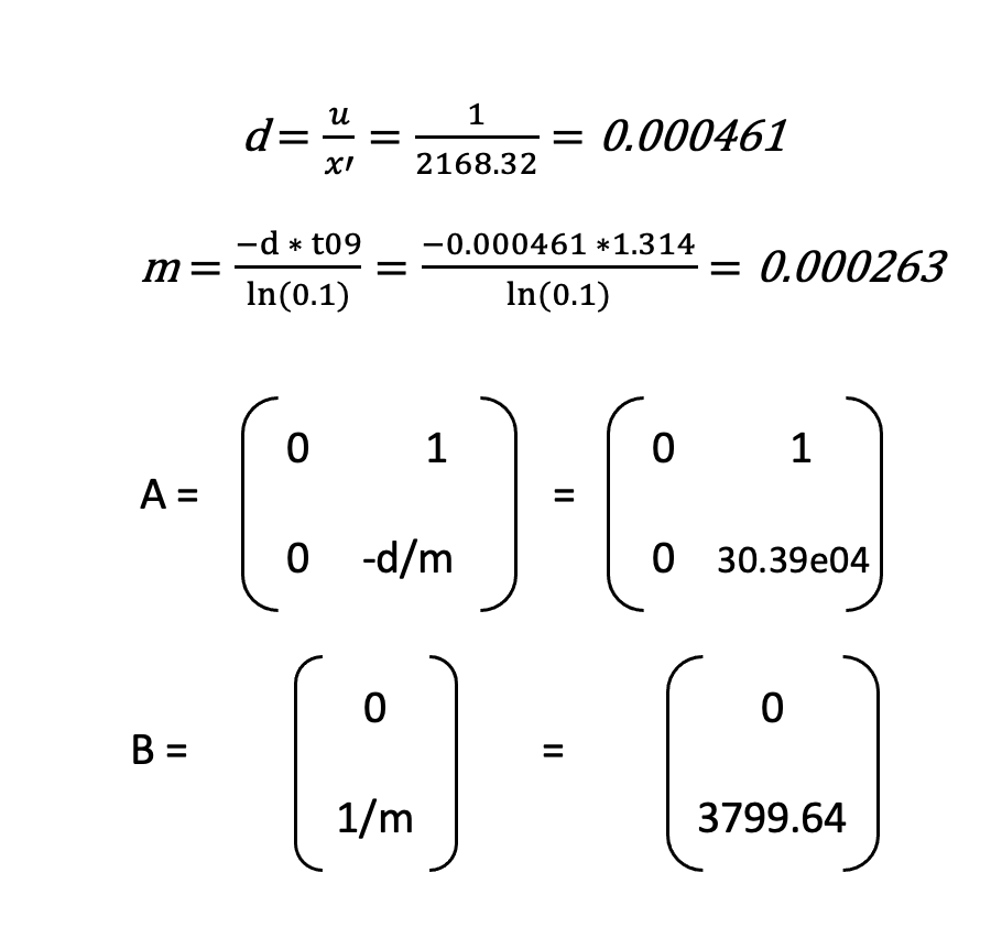
We can take the steady state speed to be -2168.32. The 90% rise time is the time taken to reach 90% of the steady state speed. We can calculate this to be t90 = time of Step Response Application – time at 90% steady state speed = 1.314.

We can compute d and m as follows. We have used u = 1, as in lecture. They can be used for A and B matrices in the state space equation.

Kalman Filter Setup

We need to define the process noise and sensor noise covariance matrices. These values will affect how much the filter trusts the prediction and the sensor measurements. For the process noise covariance matrix, we need to values sigma_1 and sigma_2 the covariance for position and speed respectively. As I wanted to test how well the model works first, I set these to be 10 each. My sensor is not very accurate, especially for long distances, so I set sigma_3, the sensor noise to be 20. Below are the two noise covariance matrices.

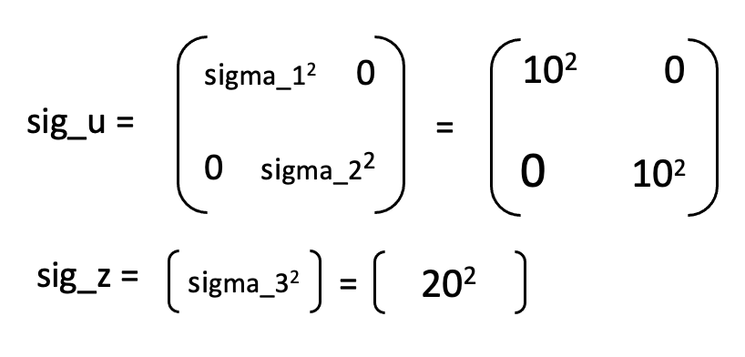
We measure one state, the distance from the wall, and our state space has two dimensions – position and speed. So, C is a 1 x 2 matrix. As the robot is moving towards the wall, the sensor measures are negative. We have to use [-1, 0] as the C matrix.

Kalman Filter in Jupyter Notebooks

We wanted to run the Kalman Filter in Jupyter Notebooks before integrating it in the robot. To do so, I modified the code to take sensor measurements when available while performing Task B. As we will use the Kalman Filter to decide when the robot should turn, I only used the distance measurements for the straight part in the beginning.

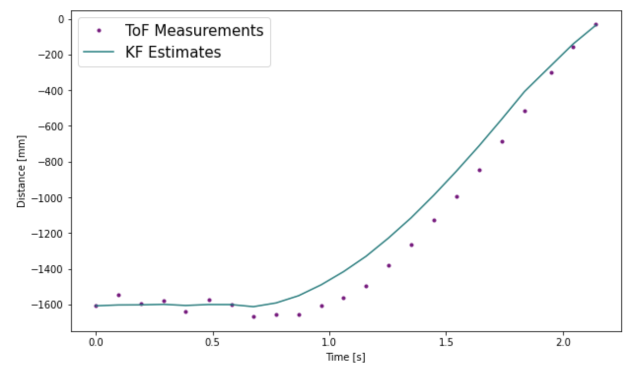
Next, I wrote a Kalman Filter function, which takes in the distance measurement and motor input, runs the prediction step and update step and returns the estimate for the sensor distance. Note, I used Delta_t = 0.096 as the sampling time. This is the average sampling time for this run. Given below is a plot of the Kalman Filter output.

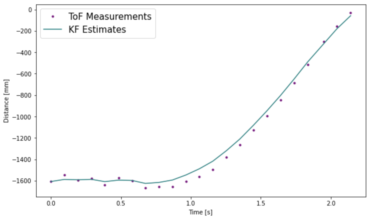
Increasing sigma_3, the sensor noise, to 50, the filter trusts the model more and does not follow the sensor values as much. It is interesting that towards the end, they both seem to coincide. This means that our model was pretty good.

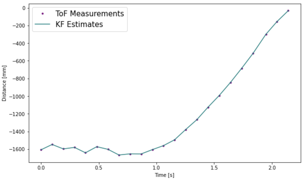
Decreasing the sensor noise to 5 and increasing the position and speed noise to 50, results in a filter and trusts the sensor values a lot more than the model so it follows the sensor measurements.

Kalman Filter on Robot

Lastly, I wrote the above Kalman Filter function in Arduino code. I used the BasicLinearAlgebra library to work with matrices. As in the python code, the sampling time used is constant. It is the sampling for taking the first measurement. I could have used the exact sampling times for each step, but this would have increased the computation time of the filter. As the sampling times were very similar in recorded runs and we needed the Kalman filter to work fast, doing this made sense.

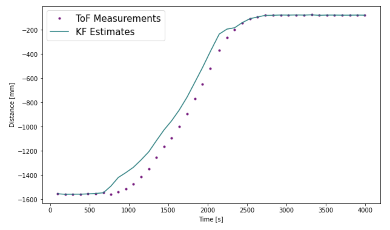
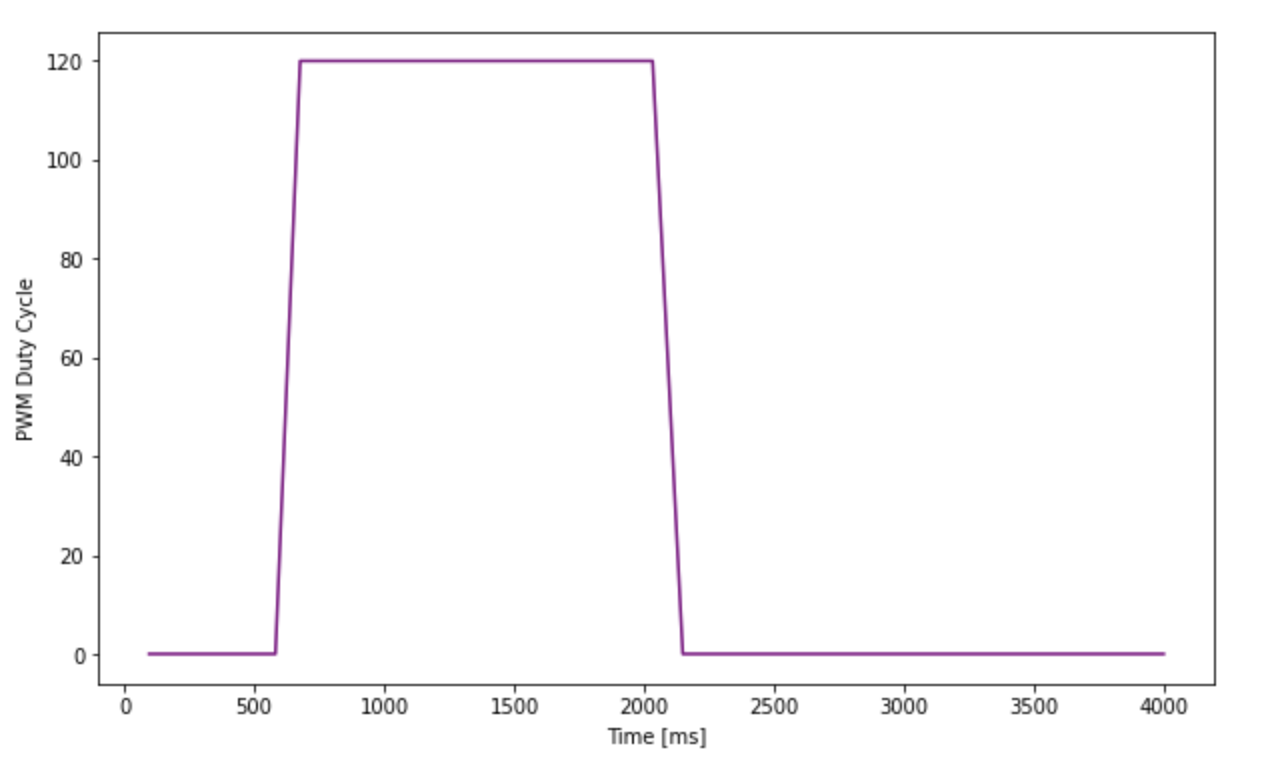
For the initial covariance variables, the Kalman Filter worked badly. Notice, as soon as the PWM motor input is set to 120, the Kalman Filter predicts that the robot moves with a very high speed at that instance as there is drastic change in distance. However, the sensor measurement does not change as much. This might be because it takes the motors a while to ramp up before they start moving due to friction of the floor. As the Kalman Filter was tuned using real data, it should have accommodated this, however the battery charge was fully charged while executing the step response, so it might have ramped up much faster.

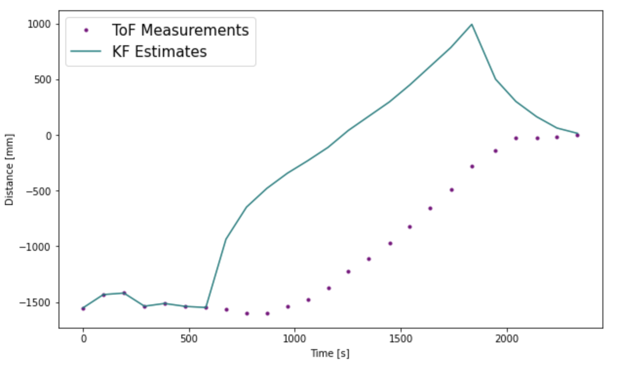
To make the Kalman Filter predictions more accurate, we need to increase the trust in the sensor readings and decrease the trust in the model. After a lot of tuning, I found sigma_1 = 60, sigma_2 = 60, sigma_3 = 20 works best. Notice in the graph before, the KF estimates are a little ahead of the sensor readings, this is means that the KF filter is predicting where the robot is.

Conclusion

I found is lab extremely tedious and time consuming. I faced a lot of issues and had to repeat multiple steps. Initially, I had set the ToF sensor timing budget to 20ms and completed the entire lab using that data. I was able to collect sensor readings every 18ms-20s, however the data was very inaccurate. I had to switch my front and side sensors midway through the lab, as the front ToF sensor stopped working due to crashing into the wall. I spent a lot of time understanding how the Kalman Filter works and tuning it. This lab really helped me gain a thorough understanding of the Kalman Filters. Thank you to the teaching staff for delaying the grading deadline and helping me through this difficult lab.