Objectives

• Implement grid localization using Bayes filter in the simulation

Overview

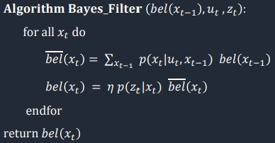
In order for the robot to determine its position somewhat accurately, we must use grid localization and Bayes filter. We split up the map into a 3D grid with coordinates (x, y, Θ). The grid will be comprised of 1944 individual cells, or each dimension will have a magnitude of 12, 9, and 18, respectively. We will be using the odometry motion and sensor model to implement Bayes filter, meaning we will be using the Gaussian Distrivbution to model the very noisy and often inaccurate odometry data (rotation1, translation, and rotation2), and update the probabilities given ToF observations. Next, we will actually implement the Bayes filter algorithm, which is shown below.

Implementation

To implement grid localization using Bayes filter, we had to complete five functions: compute_control, odom_motion_model, prediction_step, sensor_model, and update_step.

Function #1: compute_control

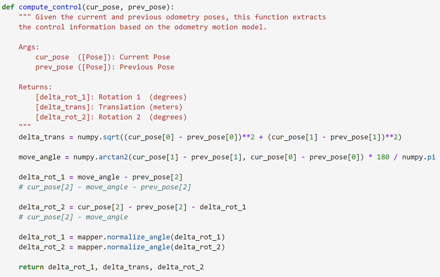
Based on the last and current odometry data which are tuples of (x, y, Θ), this function will derive the neccessaery control information, which are rotation1, translation, and rotation2. Rotation1 has units of degrees and represents the angle needed to move the previous position to point in the direction of the current position. Translation has units of meters and represents the distance needed to travel from the previous position to reach the current position. Finally, Rotation2 has units of degrees and represents the angle needed to move to point in the final direction of the current position. Below is my code of compute_control.

Function #2: odom_motion_model

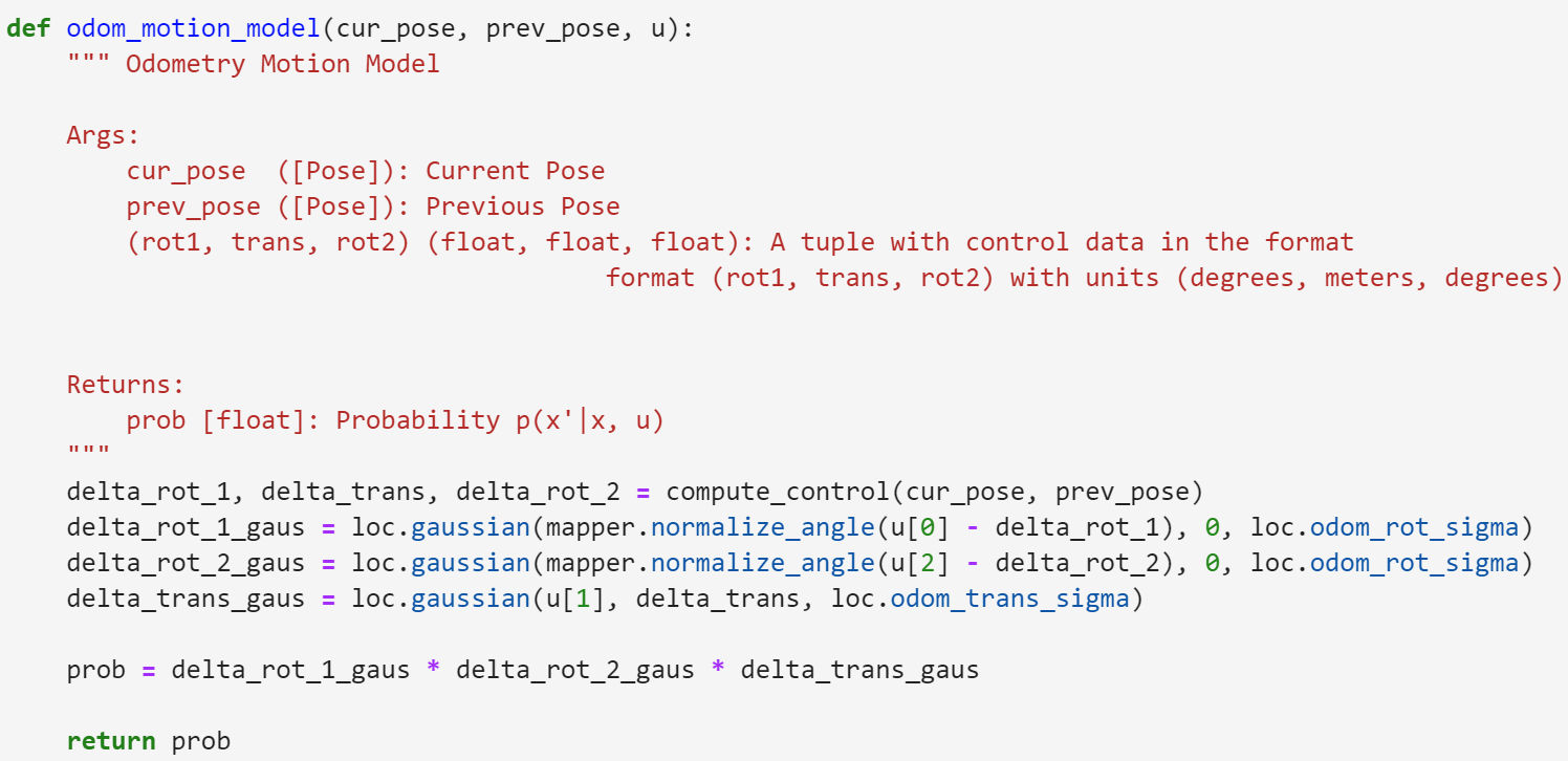
This function uses the Guassian Distribution to generate propbabilites of current measurements given the past measurements and control information of each of the dimension (x, y, and Θ). The function returns the combined probabilities of all the dimension. This function represents the transition probability or action model in the Bayes filter algorithm. Below is my code of odom_motion_model.

Function #3: prediction_step

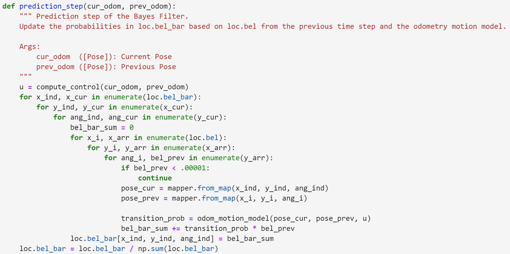
As by the name, this function represents the prediction step int Bayes filter algorithm. This function iterates though all probabilities in bel_bar, which corresponds to all the grid squares. Then iterates through all the previous bel proabilites of all grid squares to sum and update the bel_bar probability. This is the prediction step that updates based on the control input of odometry data. Below is the sudo code (highlighted in red), and my code of prediction_step.

Function #4: sensor_model

This function implements the measurement probability or sensor model part of the Bayes filter algorithm. It generates a probability array containing the repsective probabilities of each ToF sensor reading. Each probability is the likelihood of the real measuremnt given the current control input. Below shows my code of the function sensor_model.

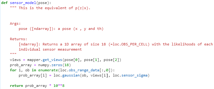
Function #5: update_step

This is the final function that combines all the past funcions to implement the totality of the Bayes Filter algorithm. Just like prediction_step, we iterate through all the bel_bar values and update the respective bel value accordingly, based on the sensor_model and bel_bar, which was already updated in prediction_step. It is also important to note that we must normalize all the bel values at the complete of the function. Below is the sudo code (highlighted in red), and my code of update_step.

Simulator

Below is a video plotting the odometry (red), ground truth (green) and belief (blue).

Below is a video plotting the odometry (red), ground truth (green), belief (blue), and the marginal distribution bel_bar(x,y) in the 2d grid space.

Important Note

I worked extensively on this lab with Joey Horwitz (jah569). His website can viewed here.