Objectives
- Wire up the sensors to the Artemis Nano
- Demonstrate ability to read data from individual sensors
- Transform data from sensors into other forms
Materials
- 1x SparkFun RedBoard Artemis Nano
- 2x Time-of-Flight sensors
- 1x 9DOF IMU sensor
- Quiic connectors and various wires
- Soldering iron, helping hands, etc
Prelab
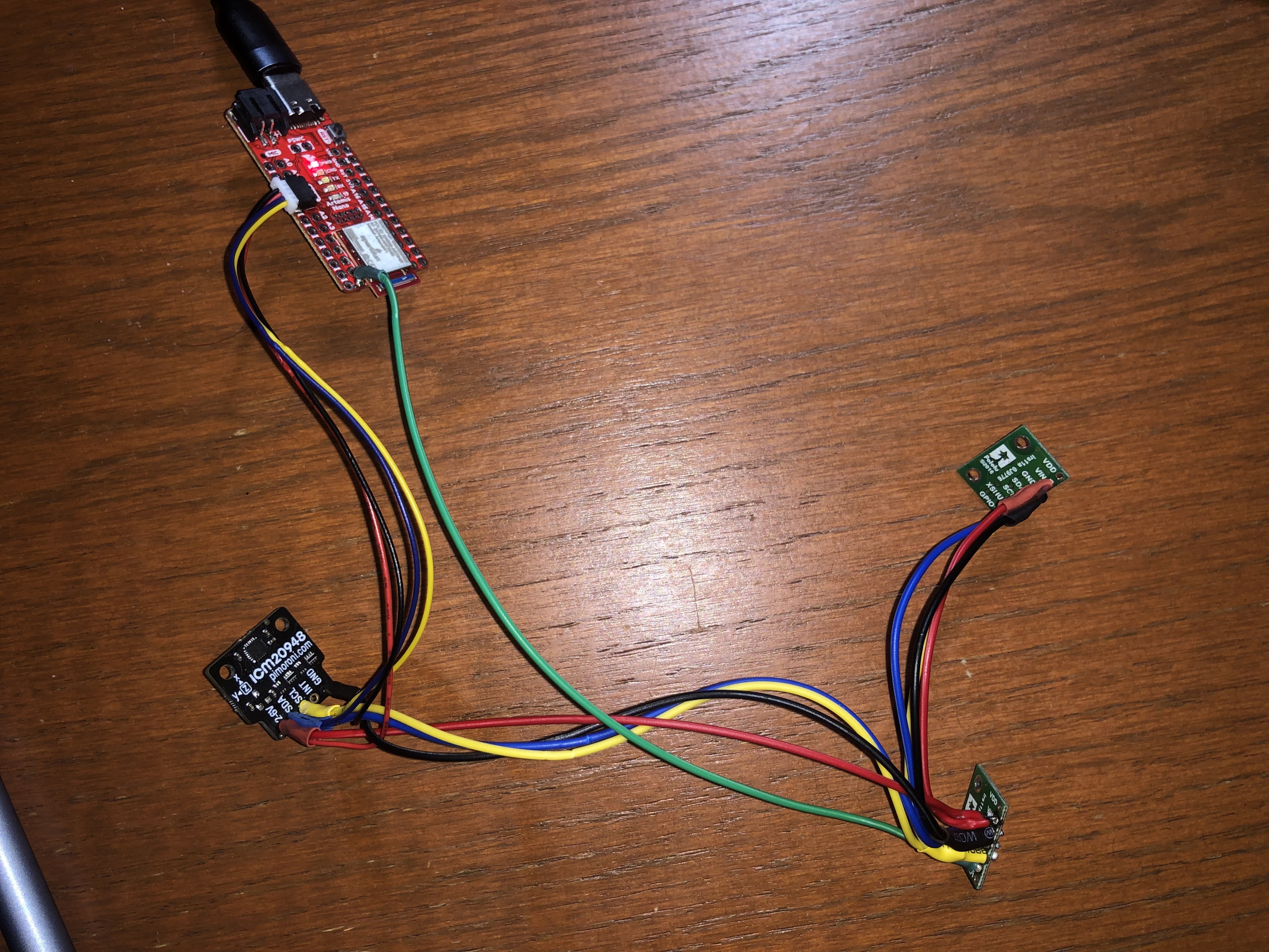
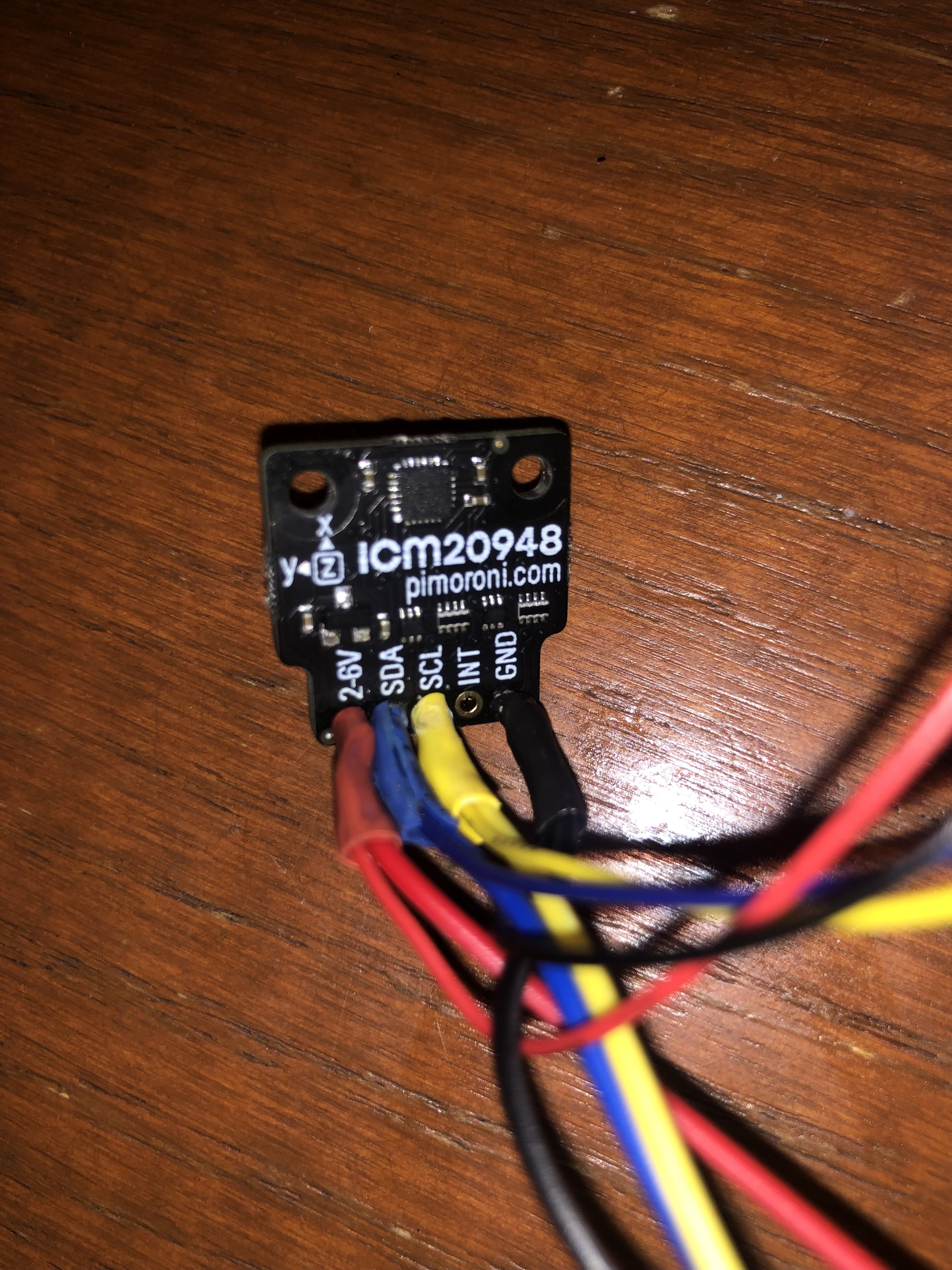
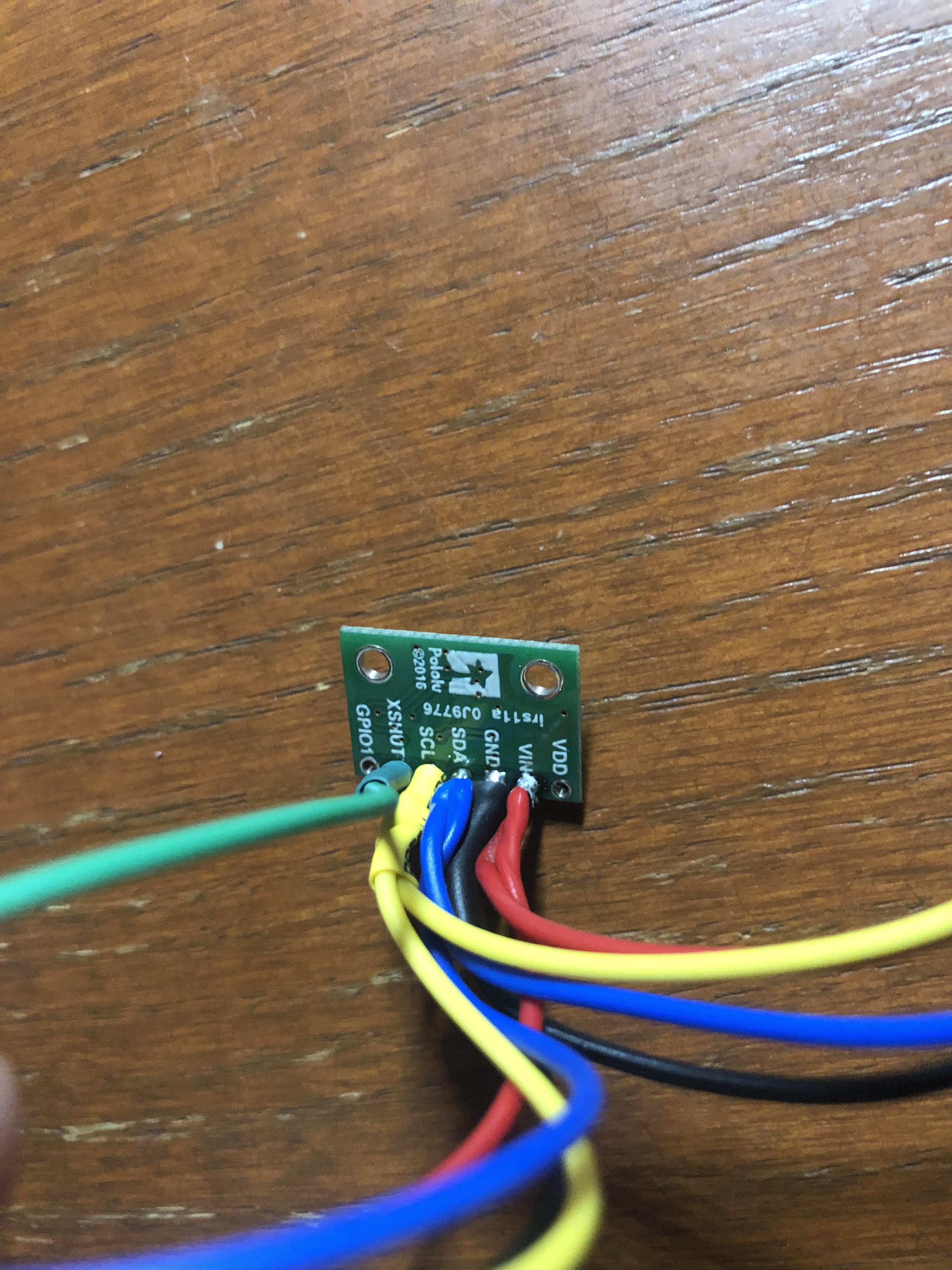
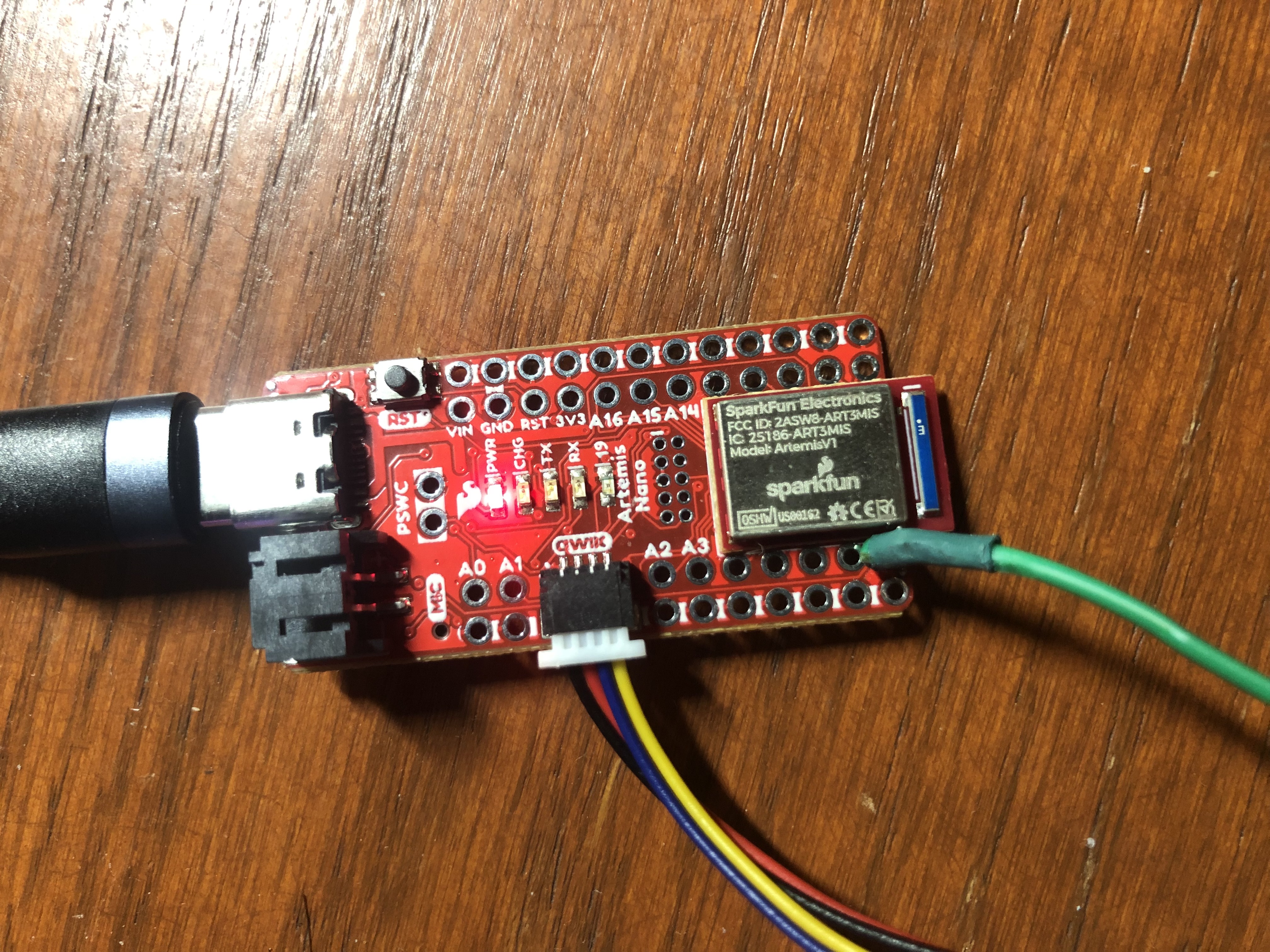
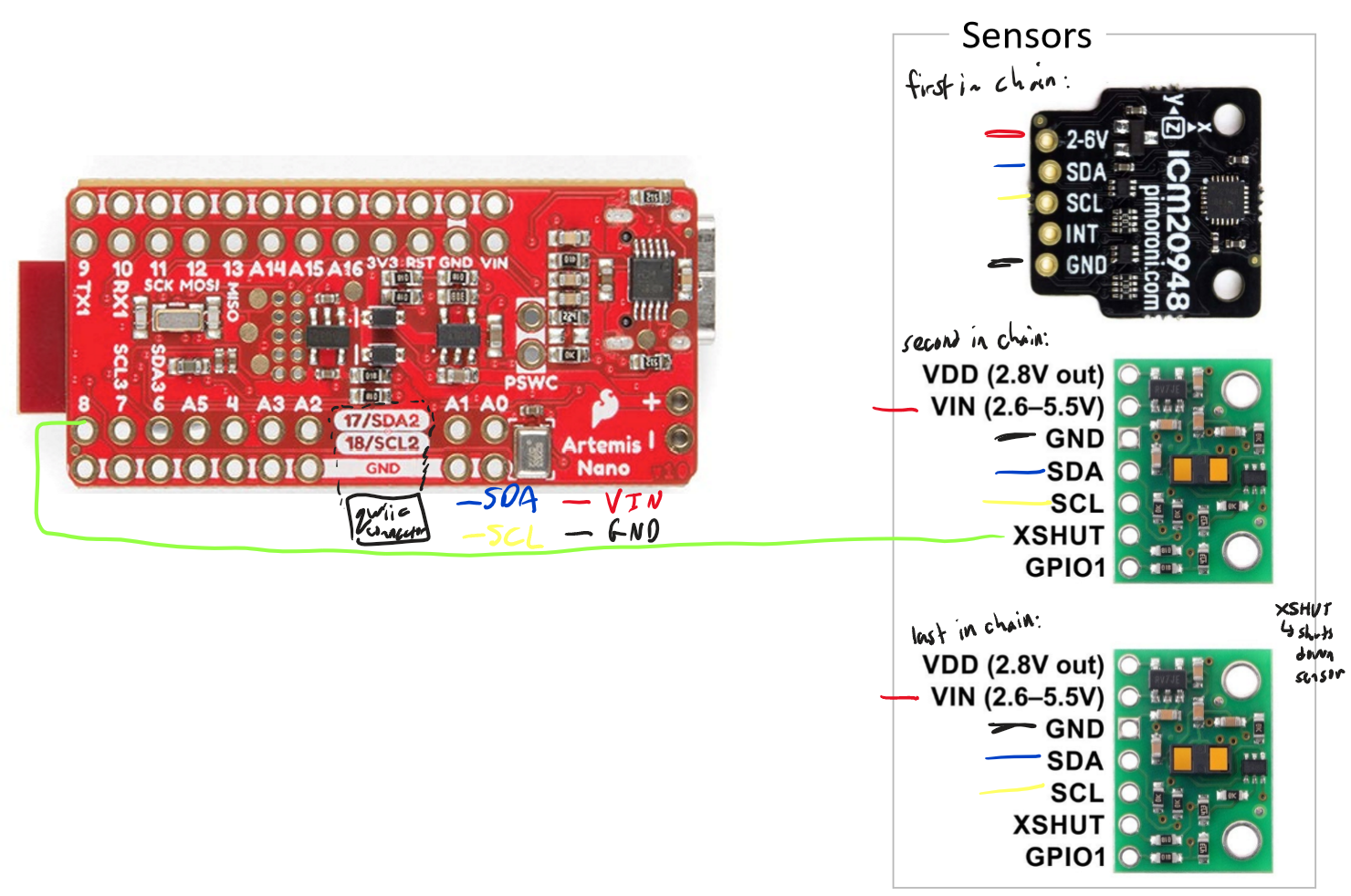
The goal of this lab is to connect the two time-of-flight sensors and the IMU sensor together by daisy-chaining the power, ground, SCL, and SDA wires. Before soldering my sensors together, I had to decide on some crucial decisions, including whether the connections would be permanent, what order the sensors would be in the chain, how long the wires would be, and how I would overcome the issue of having two identical ToF sensors. I decided that I would make all the connections permanent between the sensors because there would be no instance where I would want to disconnect them, and it would eliminate the space that would be taken up by header pins. I also decided to leave my wires substantially long because it would allow me to move my sensors into any position I would like. I recognize that the wires will take up some space in the car chassis, but I believe that the wires are small enough to fit in anywhere. I decided to solder my IMU closest to the Artemis board because it would stay by the middle of the car, and my ToF sensors farther are because they would need to be by the exterior of the car. I also intend to place my ToF sensors in the front of the car facing out at an angle because it will give the car the best vision. Finally, I decided to to the approach of only soldering one XSHUT on the ToF to the Artemis because it is simpler coding-wise and also reduces the number of wires used. Below is the wiring diagram of my sensor setup.
Time-of-Flight Sensors
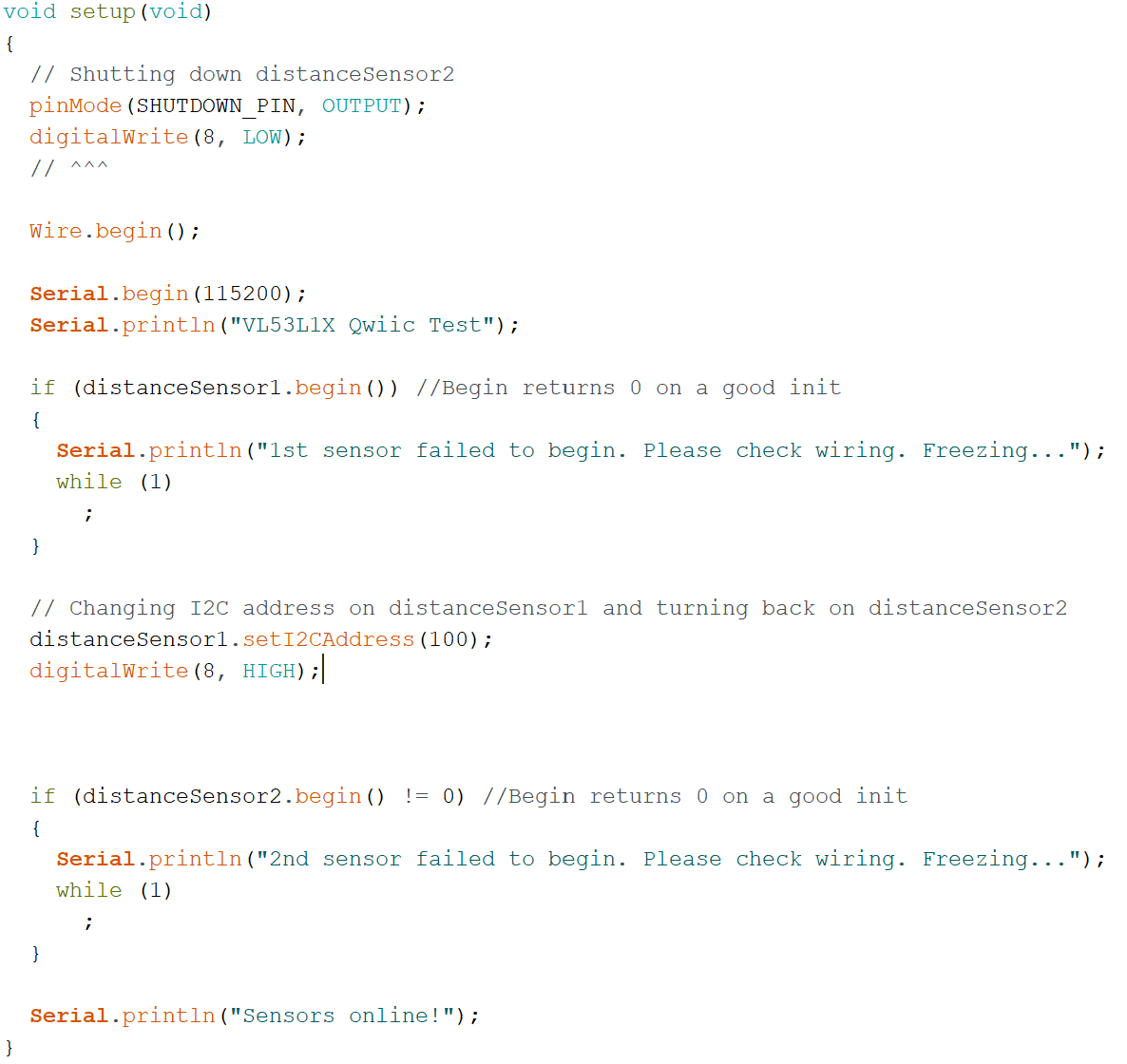
After finishing connecting all my sensors together, I began to test my ToF sensors. When running the I2C wire example, I had received a strange list of all addresses possible, presumably because there were three addresses detected instead of two, and the lab TAs said to ignore this step. As I stated in my prelab, my design decision was to use one XSHUT pin on the first ToF sensor to turn it off, then change the address of the second ToF sensor, and then turn the first ToF back on, all in setup. This way the addresses of the two identical ToF sensors would not conflict. Below is my setup code which is where this action is preformed.
My next task was to set out the different modes that the ToF sensors could be put in. One was .setDistanceModeShort() and the other was .setDistanceModeLong(). The difference between the two is as the name states. .setDistanceModeShort() can read short distances more accurately, and .setDistanceModeLong() can read longer distances more accurately. The mode I intend to use is .setDistanceModeLong() because while .setDistanceModeLong() has some inaccuracies, .setDistanceModeShort() has a max sensing range of around 1.3 meters and will not be able to give us good sensor readings in open space.
Next, my goal was to test the accuracy of my ToF sensors using .setDistanceModeLong(). Below is a graph of my findings.
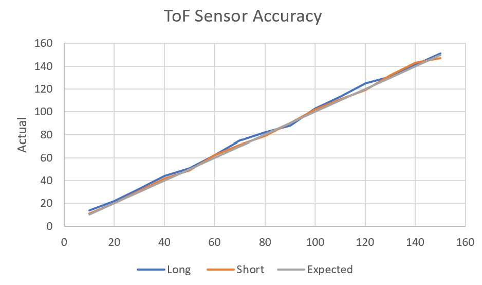
The data was fairly accurate, as shown by the graph. I also tested the ToF sensors against a dark and light background and could not distinguish a difference between the two, nor could I distinguish a difference between a smooth and rough texture. Please note the video below showing that two ToF sensors were effectively used at once.
IMU Sensor
After connecting the IMU to the Artemis board using I2C wiring, I ran the example basics to ensure it was running properly. Before uploading the code, I made note of the AD0_VAL definition, which represents a bit in the address which determines whether you are writing or reading data to the IMU. For our purpose, we will be exclusively reading data from the IMU which means AD0_VAL should be 0. I uploaded the code, and below is a video of the data when I move the IMU around in various motions. The accelerometer data is given in mg (or micro-g), the gyroscope data is given in DPS (or degrees per second), and the magnetometer data is given in μT (or micro-Telsa). From the serial plotter, the data lined up with the motions I was performing.
Accelerometer
My next task was to use the accelerometer data to derive pitch and roll. Below is a code snippet of the equations I used to do that.

Below is my experimental data showing both pitch and roll values as the IMU moves from -90 degrees to 0 degrees to +90 degrees. The first picture shows pitch data, and the second shows roll data.
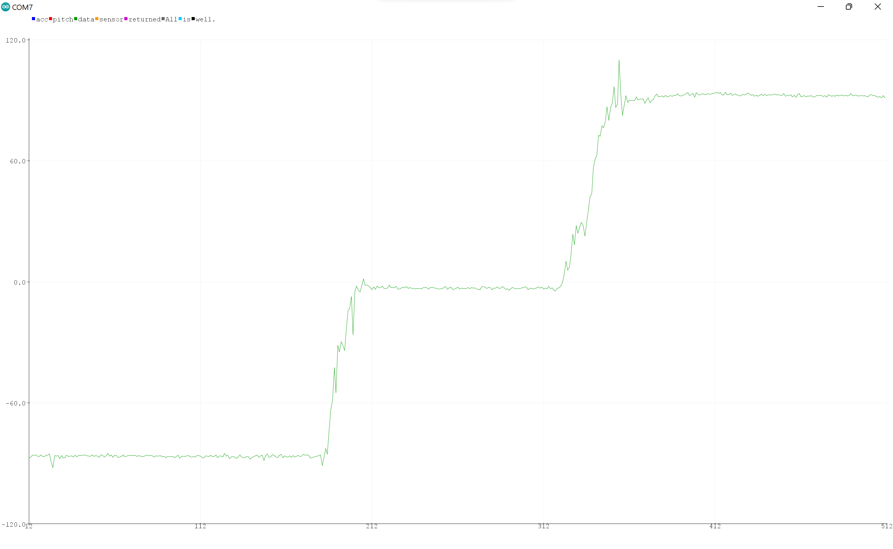
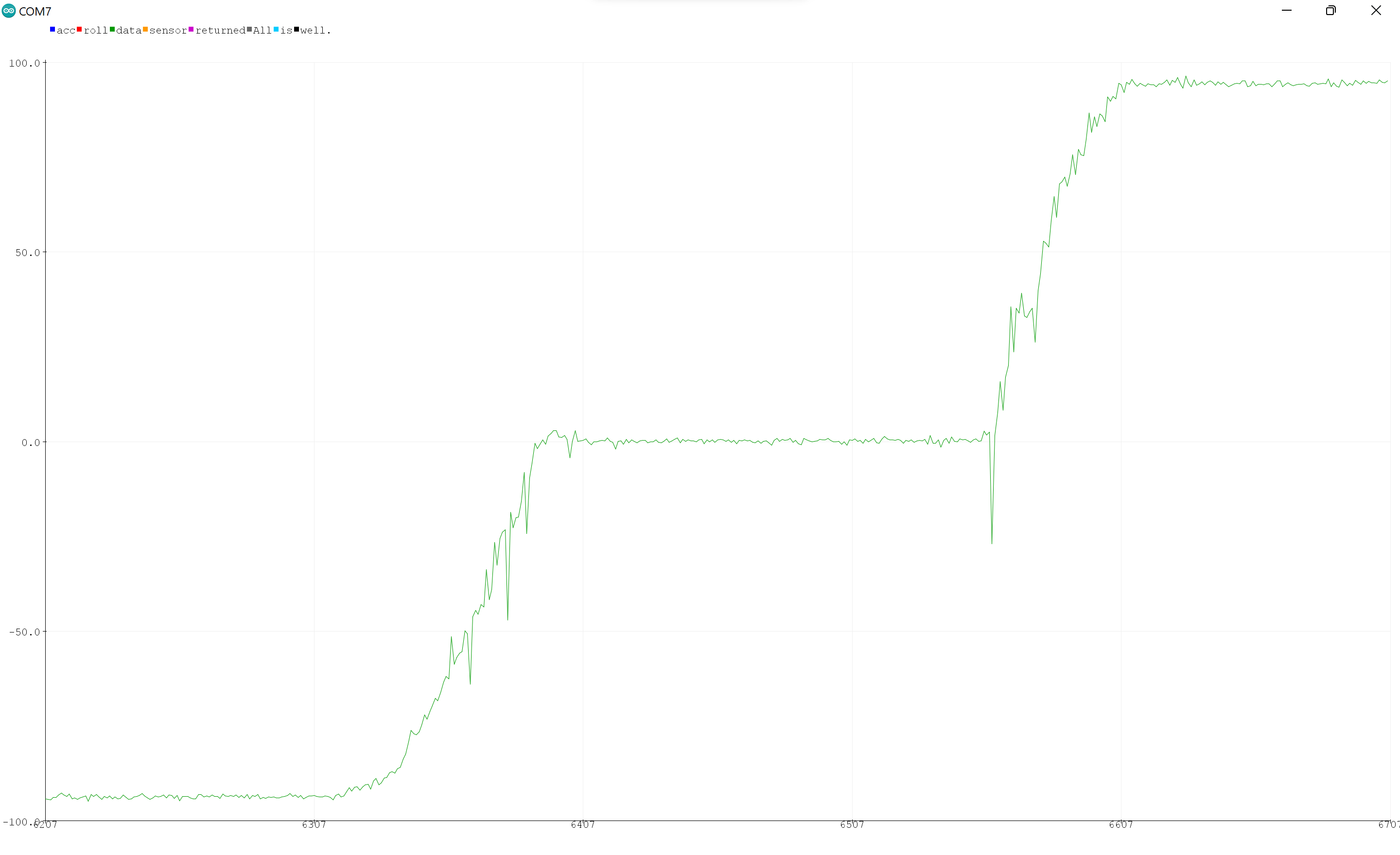
As the serial plotter shows, the data is fairly accurate, except for the large variations while moving (caused by noise). The actual values fluctuate around the expected value with a maximum deviation of around +/-1.5 degrees, giving us a percent error of around 1.67%.
I preformed a FFT analysis on the noise created by slightly tapping the IMU. Below are my graphs of the signal generated by the tapping, and the corresponding FFT graph.
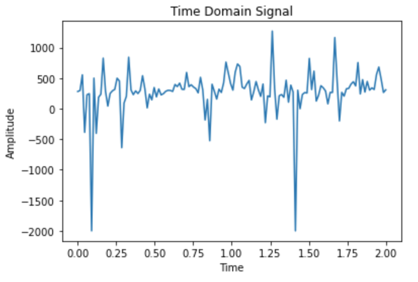
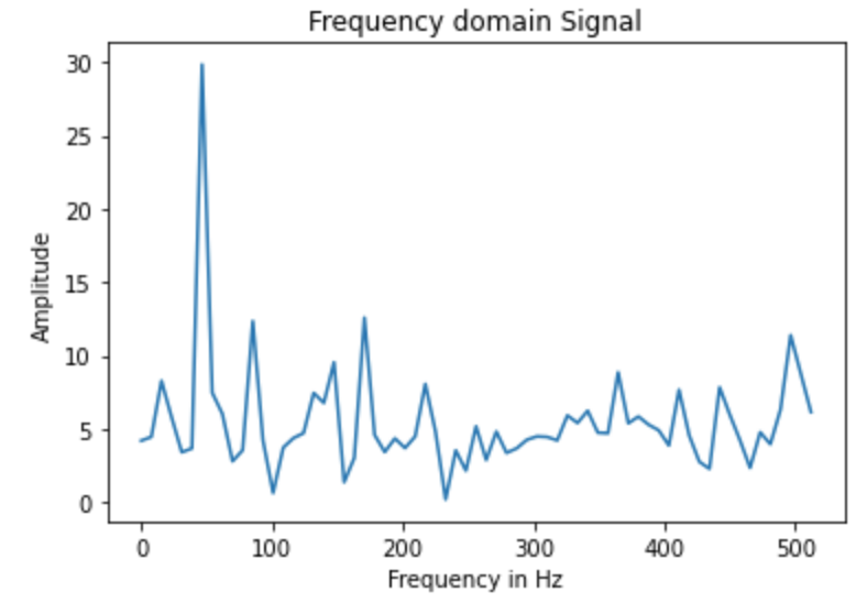
As you can see, the noise frequency occurs most around the frequency values of 0-100Hz, so creating a low pass filter eliminating these frequencies would significantly reduce the unwanted noise. The cutoff frequency will reduce the accelerometer data values that occur when small variations of unwanted noise occur, so the end result will be data that is more accurate and stable.
Gyroscope
Moving onto the gyroscope, I was tasked to use equations learned in lecture to compute pitch, roll, and yaw angles from the gyroscope data. Below is a code snippet of how I implemented these functions, followed by the serial plotter of that derived data.

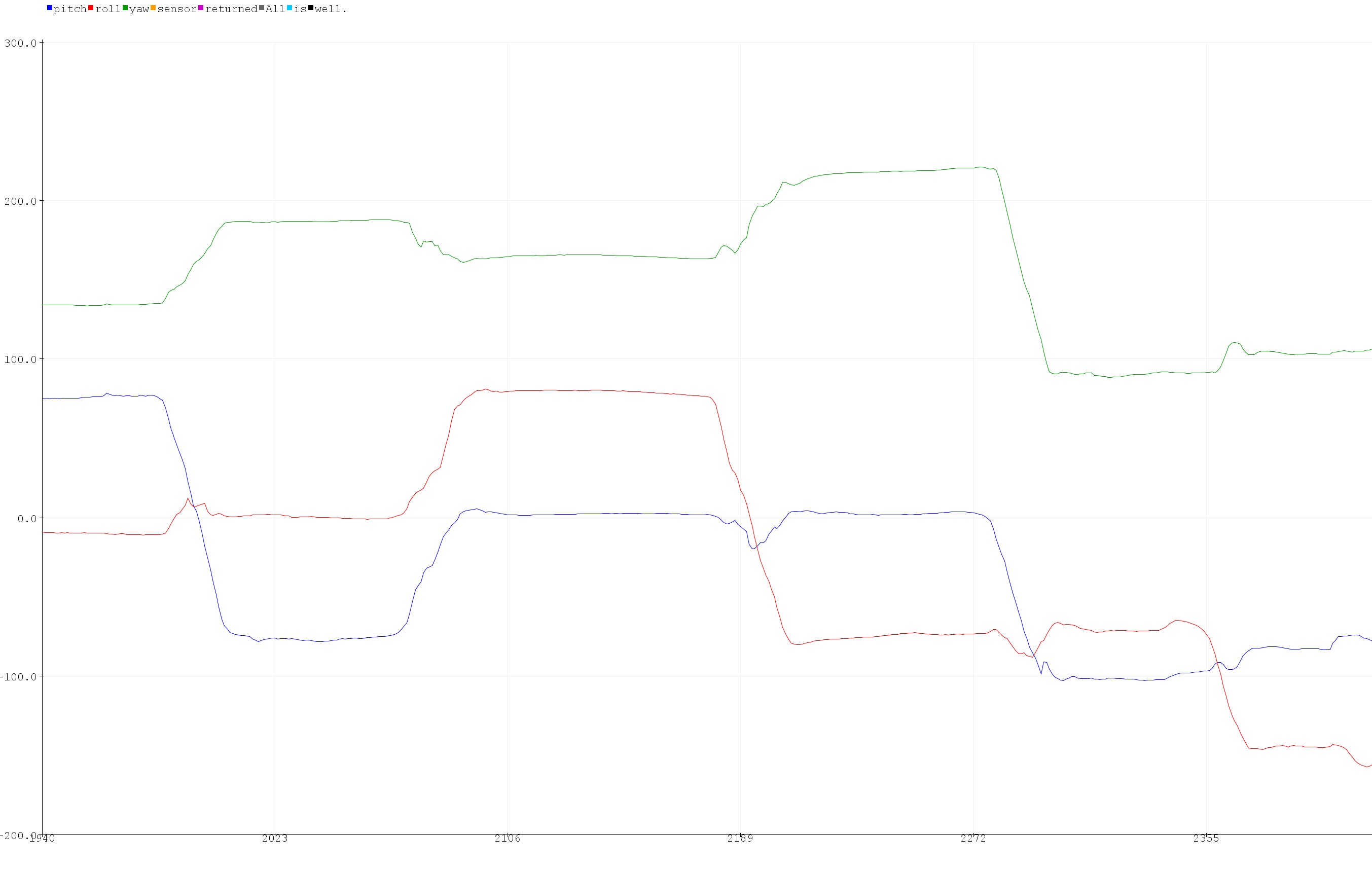
Deriving the degrees from the gyroscope results in fairly accurate data corresponding to the movements I made; however, drift occurs from unwanted noise from the raw gyroscope data, which effects the calculated degree. Overall, the degrees derived from the gyroscope is much smoother than when derived from the accelerometer, but the accelerometer derived data seemed to be more accurate. Below is a graph of the general drift that occurs, even when no movement occurs.
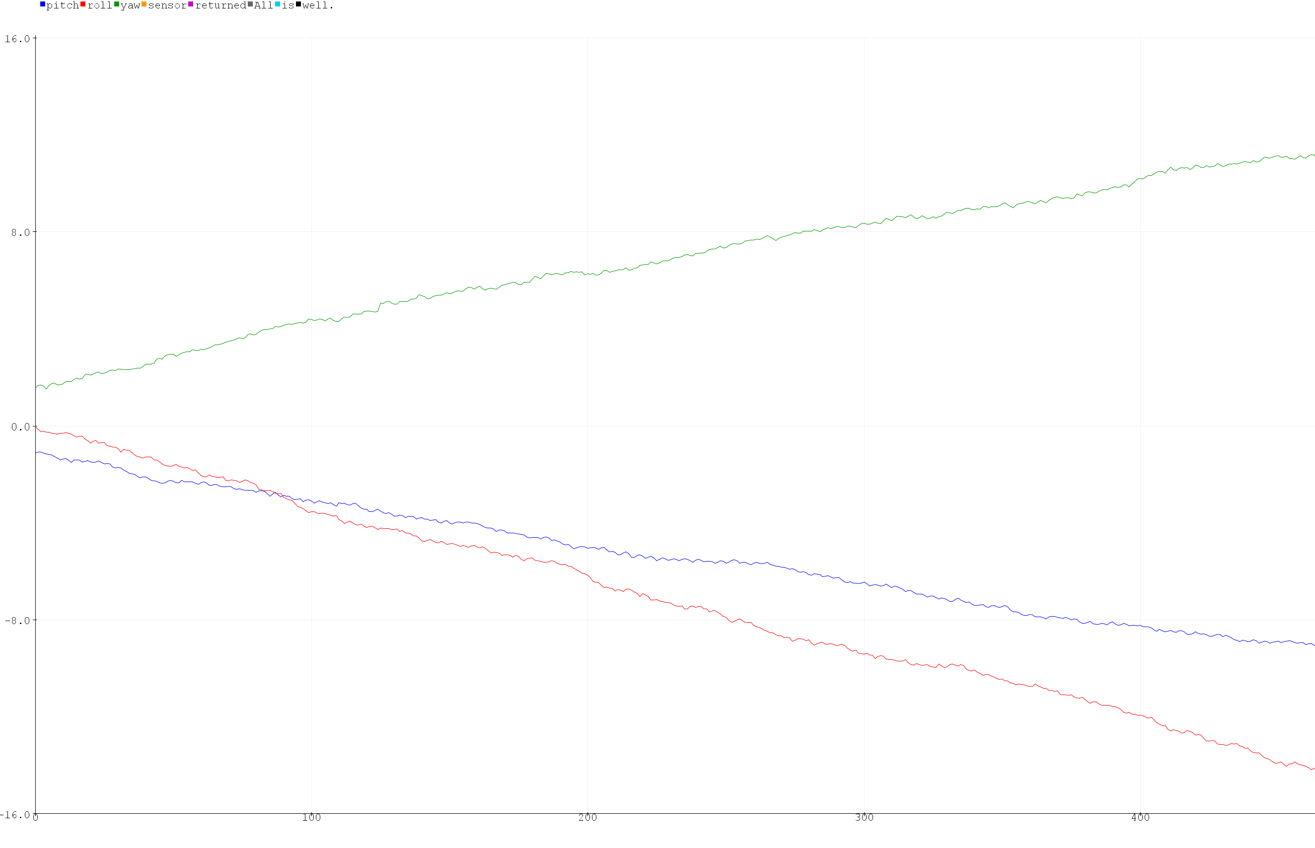
The drift is actually very significant, so it is important that we implement the complementary filter to reduce it. I changed the sampling frequency from 15ms to 30ms to 60ms, which changed the actual drift that occured, although those differneces were very small. Decreasing the frequency, resulted in less drift, while increasing the frequency resulted in more drift. Although, the smaller sampling frequency, seemed to have more inaccuracies.
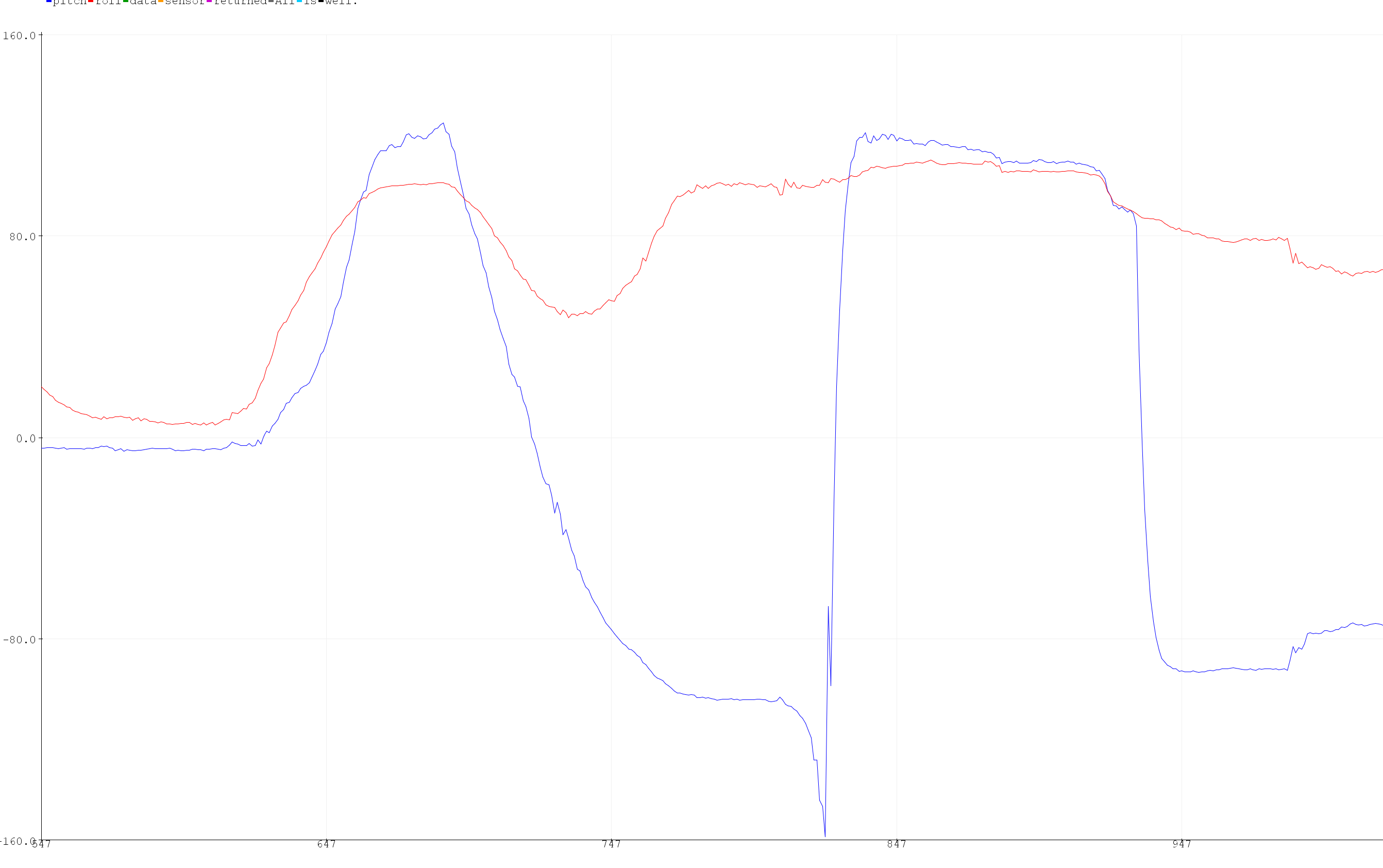
To get the best of both worlds from each technique of derivng the degrees from each axis, I implemented a complimentary filter. I chose a alpha value of .3, through trial and error, and looking at which alpha value gave the best looking data. A lower alpha value gives you more empahsis on the gyroscope data (less vibrations from accelerometer), and a higher alpha value gives you more emphasis on accelerometer data (less drift from gyroscope). As you can tell by the graph below, it is not susceptible to drift or quick vibrations. My code snipet is is also included below.

Wiring Gallery
