Fig. 1. Low-pass RC circuit model in LTSpice. Image taken from lab 3 handout authored by Carl Poitras.
In lab 3, we implemented and tested a bandpass filter that will be used on our robot in the upcoming lab 4. We explored both passive and active filters that may serve this purpose. We accomplished the following tasks:
This lab 3 report will therefore be organized into 6 main sections, each discussing one of the tasks above. The Discussion section at the end recaps the goals of this lab.
LTSpice is a analog circuit simulator. The purpose of using LTSpice in this lab is to build the passive RC high pass and low pass filter as well as the active band pass filter in LTSpice, simulate their frequency response, and compare the simulation with experimental data that we measure with the Arduino.
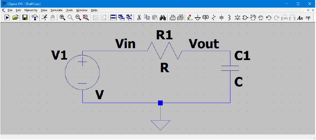
LTSpice is fairly easy to use. To simulate a circuit, we need to first build the circuit (Fig. 1). Fig. 1 shows the circuit model of the RC low pass circuit model, and it is the same process with the high pass and the band pass filter.
Fig. 1. Low-pass RC circuit model in LTSpice. Image taken from lab 3 handout authored by Carl Poitras.
After building the circuit model, we need to specify the input waveform and the simulation configurations. This is specified by SINE(0 1 1KHz) AC 1 0 and .ac dec 100 1 10000 pragmas in Fig. 2.
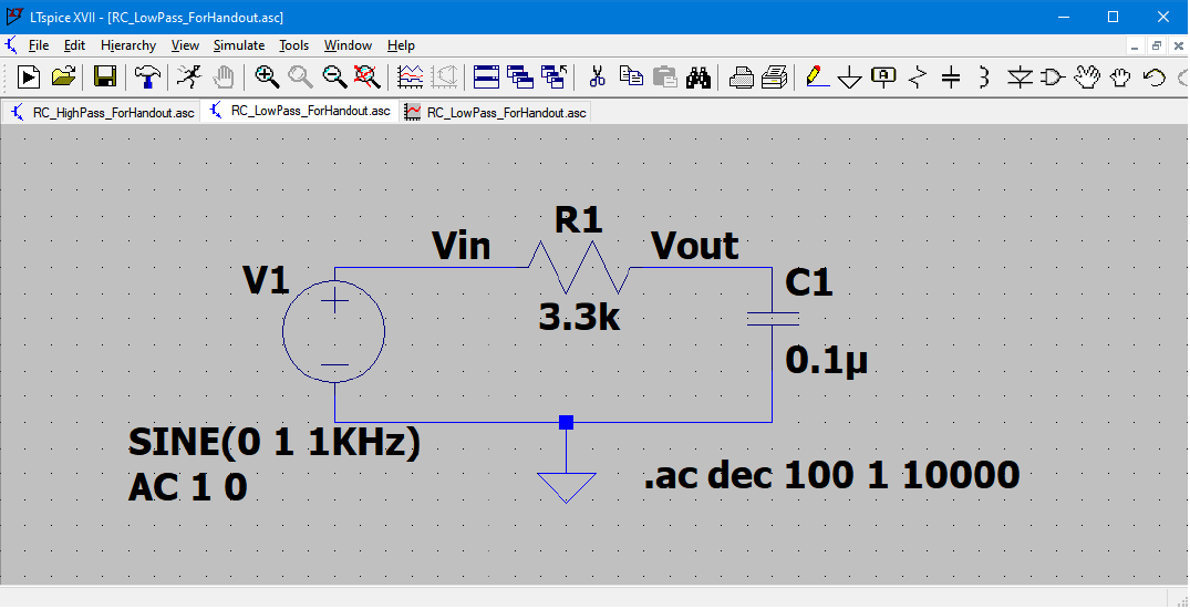
Fig. 2. Low-pass RC circuit model in LTSpice with waveform and simulation config pragmas. Image taken from lab 3 handout authored by Carl Poitras.
After setting up the circuits, we can run the simulation in LTSpice. Because we have specified Vin and Vout, and we have configured for a frequency sweep from 100 Hz to 10000 Hz, we get Fig. 3 as the output plot when zoomed into the cutoff frequency (-3 dB) (we need to manually select Vout as the output). We then can obtain the cutoff frequency of the lowpass filter, which is 1323.16 Hz. Frequency above 1323.16 Hz will ideally be suppressed in magnitude
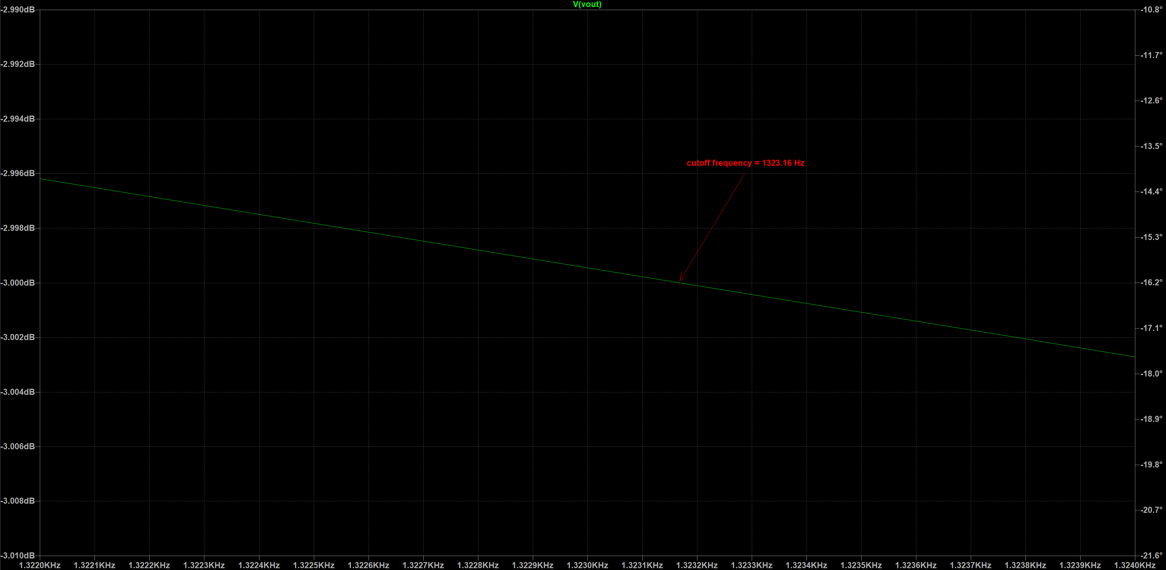
Fig. 3. Low-pass RC circuit frequency response produced by LTSpice.
Same procedure was performed with the canonical RC high-pass circuit. The RC high-pass filter was obtained by switching the position of the resistor and the capacitor in Fig. 1 and 2 without changing the position of Vin and Vout. Fig. 4 shows the simulation result of that as well. Because we did not change the resistor and the capacitor value, it is expected that the curoff frequencies for these two filters are close to each other, which is what we are observing according to Fig. 3 and Fig. 4.
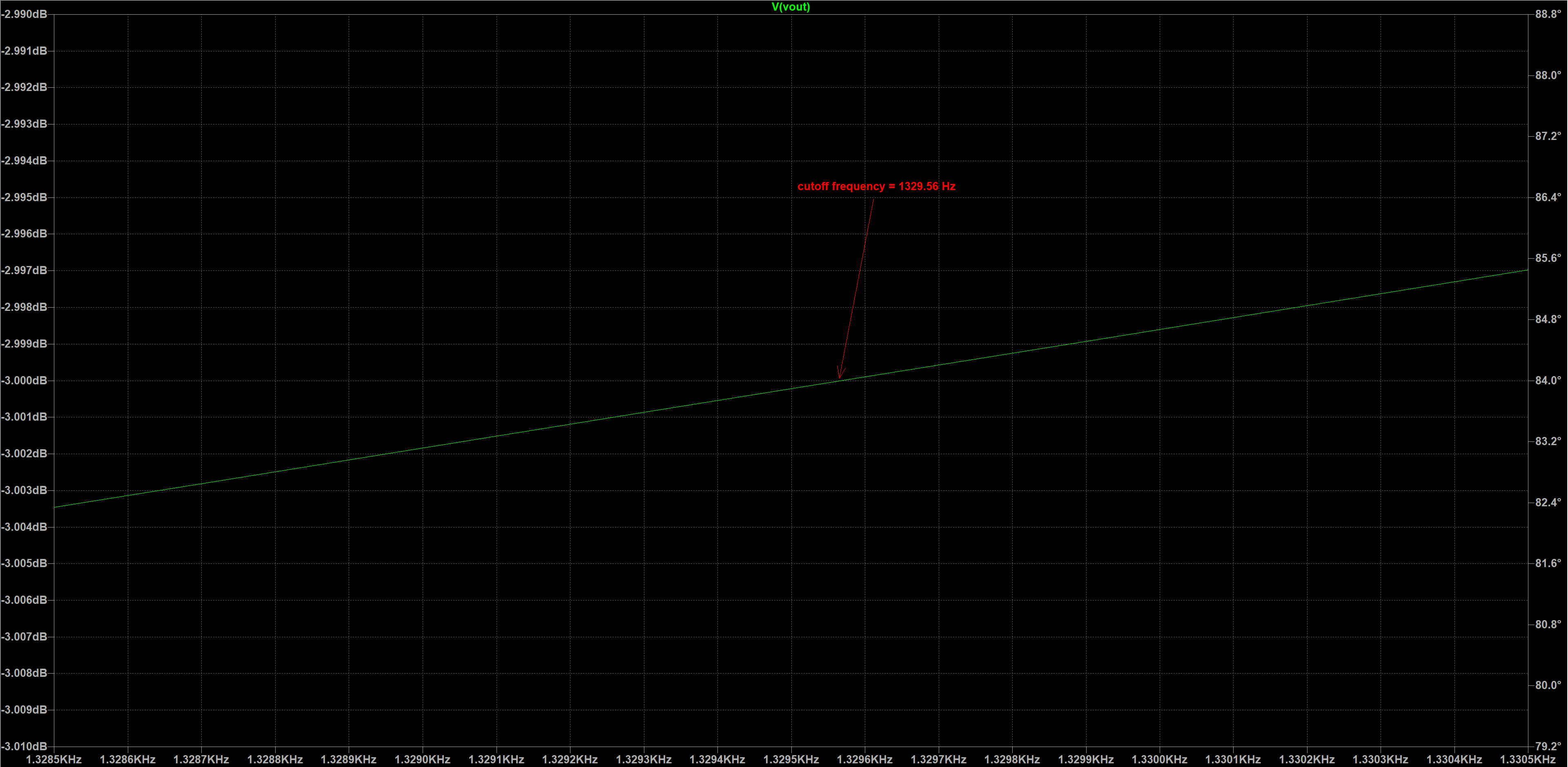
Fig. 4. High-pass RC circuit frequency response produced by LTSpice.
These simulations from Fig. 3 and Fig. 4 set a theorectical standard for us so that we can compare the actual measured RC filter performance with this theorectical prediction in later steps and determine what is a good filter for lab 4.
To measure the actual performance of the RC filters, we plan on using a microphone to perform a frequency sweep. Ideally, we can play a sound signal with varying frequency with our computer speaker, then the Arduino can use its ADC to keep sampling the output of the microphone, and send it to our computer using UART. Our computer will be running MATLAB, reading the ADC values from the Arduino, and perform FFT to identify the frequencies of sound present in the environment and picked up by the Arduino.
To do that, we need to first build a microphone circuit. We started off with a simple microphone circuit shown in Fig. 5 with R1 = 3.3 kOhms and C1 = 10 uF. The voltage on the Arduino analog input side changes when the microphone is picking up sound, which results in change of impedance of the microphone. Our Arudino will therefore use the ADC to convert the varying analog signal into digital signal recognizable for our program.
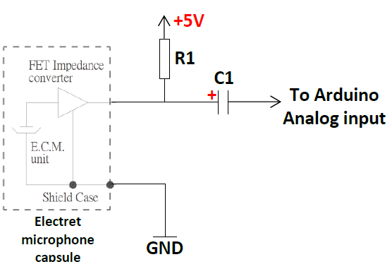
Fig. 5. Simple microphone circuit diagram. Image taken from lab 3 handout authored by Carl Poitras.
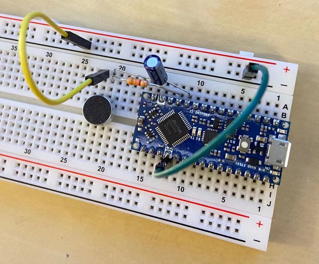
Fig. 6. Simple microphone circuit integrated with the Arduino on a breadboard.
Now that the microphone circuit is ready, we need to program the Arduino so that it does the following tasks:
With the code example 9-2 in “Getting started with ADC” PDF, we can easily adapt the ADC0_setup(), ADC0_conversionDone(), and the ADC0_read() function for our use. The ADC0_setup() is most critical because we will need to change the ADCMUX, clock divider, and the reference voltage. At the end, I was able to achieve the code below to set up the ADC when I am using AIN[3], PIN14 for the analog input pin.
// setup ADC in free running mode - AIN3 - PIN14
void ADC_freerunning_setup(){
  // setup ADC into free running mode
  /* Disable digital input buffer */
  PORTD_PIN3CTRL &= ~PORT_ISC_gm;
  PORTD_PIN3CTRL |= PORT_ISC_INPUT_DISABLE_gc;
  /* Disable pull-up resistor */
  PORTD_PIN3CTRL &= ~PORT_PULLUPEN_bm;
  ADC0.CTRLC = ADC_PRESC_DIV16_gc /* CLK_PER divided by 16 */
  | ADC_REFSEL_VDDREF_gc; /* Internal reference */
  ADC0.CTRLA = ADC_ENABLE_bm /* ADC Enable: enabled */
  | ADC_RESSEL_10BIT_gc; /* 10-bit mode */
  /* Select ADC channel */
  ADC0.MUXPOS = ADC_MUXPOS_AIN3_gc;
  /* Enable FreeRun mode */
  ADC0.CTRLA |= ADC_FREERUN_bm;
  /* Start conversion */
  ADC0.COMMAND = ADC_STCONV_bm;
}
With ADC0 set up, coding up the rest is just a trivial matter. One tricky part is to convert the ranged 0-1024 ADC reading to a signed 16-bit number. This is done by first subtracting 512 from the ADC reading to center it around 0 (counverted to signed 10-bit number), and scale the number by left-shifting the value 6 bits to make it a 16-bit value. All that is left is to connect the Arduino, along with the microphone circuit, to the computer using USB, and use MATLAB along with the Arduino to perform FFT and test the microphone circuit.
The MATLAB code backbone was provided by course staff. The backbone does the following:
This is readings from the time-domain, we will need to perform fourier transformation to see what frequencies are presented within this time domain signal. To do that, we use fast fourier transform (FFT) algorithm. Therefour, our matlab code will need to:
Fs = 1/(timeDurationofDataRead / Number of data points)abs(fftshift(fft(dataDoubleArray, Number of data points))) in MATLAB(0:N/2) * (Fs / N)One understand how FFT works, coding it in MATLAB is a trivial matter. Fig. 7 shows the time domain and the frequency domain signal from the microphone circuit when playing a 500 Hz sound from the computer speaker. We can see that although the time domain signal does not quite make sense (because of glitches in the UART communication between the Arduino and the computer), the frequency domain clearly shows a peak of magnitude in 500 Hz, meaning that the sound played by the computer is picked up by the microphone, and the Arduino ADC picks up the signal from the microphone circuit and successfully passed that signal to MATLAB, and MATLAB was able to perform FFT correctly to recover the frequency spectrum of the signal. Isn’t that amazing? Note that in the plot, we ignore the first 10 elements in the frequency domain array to avoid a huge peak at 0 Hz (which is expected because of the non-zero offset) to better visualize the peak at 500 Hz.
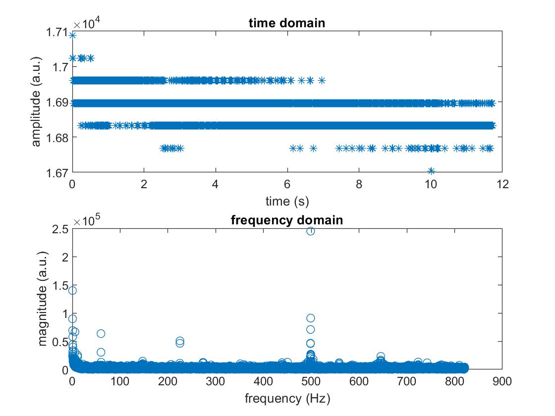
Fig. 7. Time domain and frequency domain from the microphone circuit when playing a 500 Hz sound. Plot made with MATLAB.
Now that we have our tools ready (Arduino, Microphone circuit, MATLAB), we can build different circuits and amplifiers on top of the microphone circuit and measure how that changes the frequency spectrum for different frequencies of sound played!
From Fig. 7, we can see that the spectrum’s value at 500 Hz is relatively weak, this is because the microphone is not good at picking up sound, the interference (possibly from jumper wires and breadboards, or internal in the Arduino) noise also join and makes the 500 Hz signal relatively weak. Therefore, we first try to add an amplifier to see how it can amplify the signals coming from the microphone and possibly give us better results in picking up the 500 Hz signal.
The amplification circuit, along with the microphone circuit, is shown in Fig. 8. We use an op-amp (LM358) in negative feedback mode to provide gain for the input signal coming from the original microphone circuit. After amplification, we can hopefully get a more obvious peak in the spectrum when the Arduino analog input is connected to the output of the amplification circuit. The assembled circuit along with the Arduino on the breadboard is shown in Fig. 9.
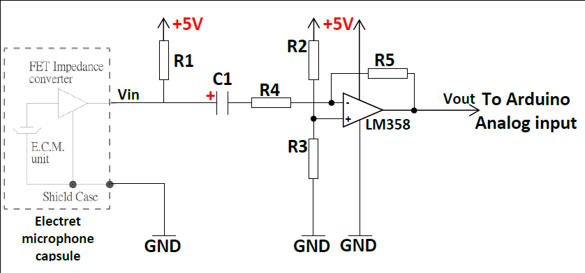
Fig. 8. Circuit diagram of microphone circuit along with amplification circuit. Image taken from lab 3 handout authored by Carl Poitras.
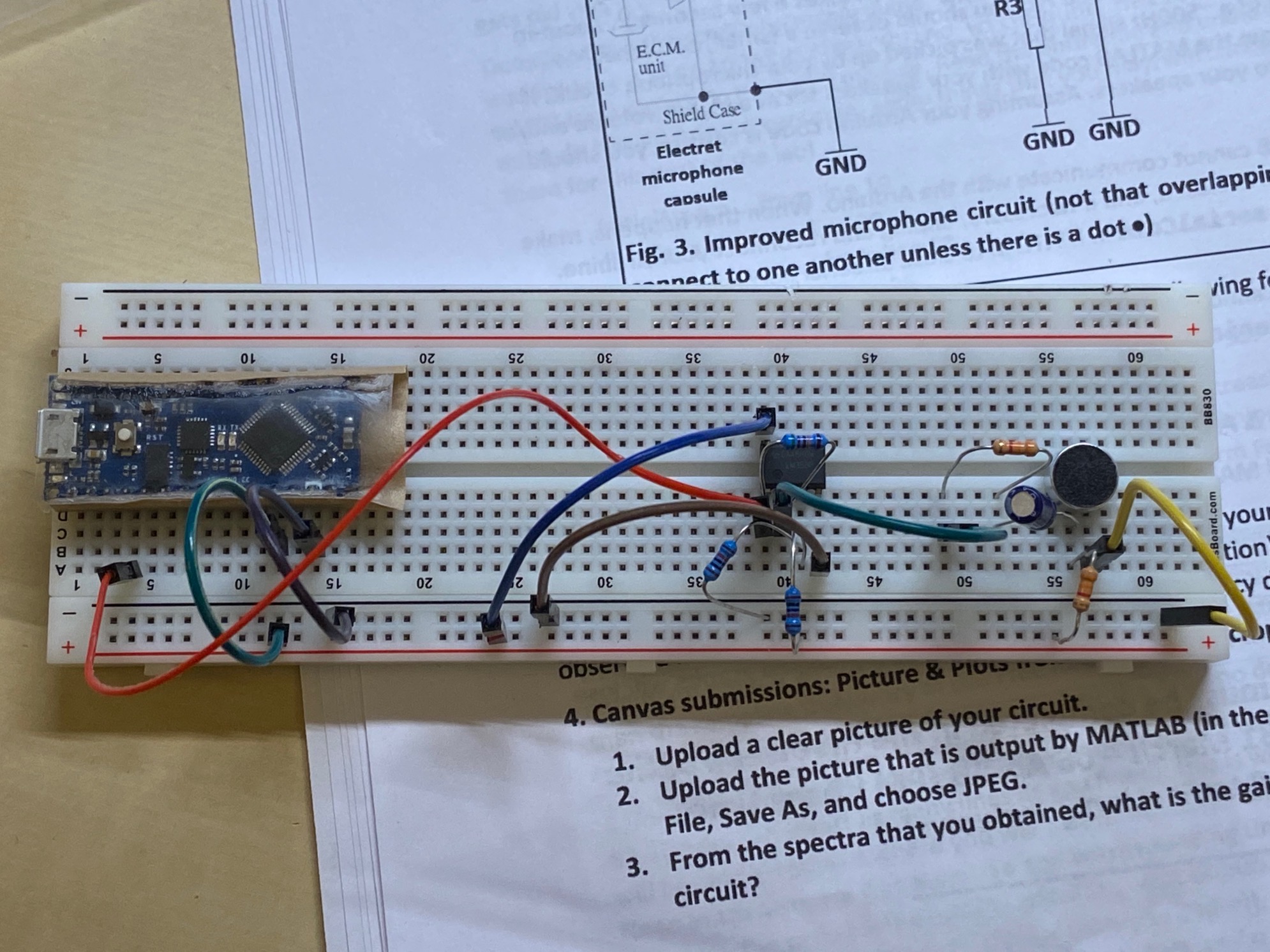
Fig. 9. Microphone circuit along with amplification circuit on the breadboard withe the Arduino.
We then simply repeat the process in the previous section. We play a 500 Hz sound with the computer, let the Arduino (now with amplification circuit) pick up the sound, the Arduino converts the ADC readings to signed 16 bit values, and MATLAB on the computer collects the data, performs FFT, and generats Fig. 10.
From Fig. 10, we can see that the 500 Hz peak is much more obvious. In Fig. 7, we can see peaks ~200 Hz and 650 Hz, and now they are gone. We still see the ~50 Hz peak, which could be background noise present in the environment and also picked up by the microphone. However, we have succeeded in amplifying the microphone circuit output with our amplification circuit for the frequency range of interest!
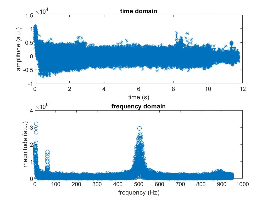
Fig. 10. Time domain and frequency spectrum for microphone circuit along with amplification circuit picking up 500 Hz sound signal played by the computer speaker.
The next step is to add in the low pass, high pass, and band pass filters, and compare the theorectical performance predicted by LTSpice with the measured performance. The connection configuration is as followed: Micrphone circuit -> amplification circuit -> filter -> arduino analog input. In this section, we are not only playing 500 Hz signal. Rather, we play a sound signal from 200 Hz to 1500 Hz to cover a wide frequency. By doing this, we can first measure the frequency spectrum with the signal coming out from the filter, and divided that by the frequency spectrum of signal coming into the filter. This way, we can recover the actual frequency response and compare that with the theorectical prediction made by LTSpice.
In addition to modifying the circuit, we also need to modify the MATLAB code to adapt to the following things:
For the low pass and the high pass filter, we use our previously simulated passive RC filters. For the bandpass filter, we went fancy and used the 4-pole Butterworth bandpass filter (Fig. 11) that consists of two op-amps. The filter should have unity gain, bandpass center frequency of 700 Hz, and bandpassing starting from 400 Hz.
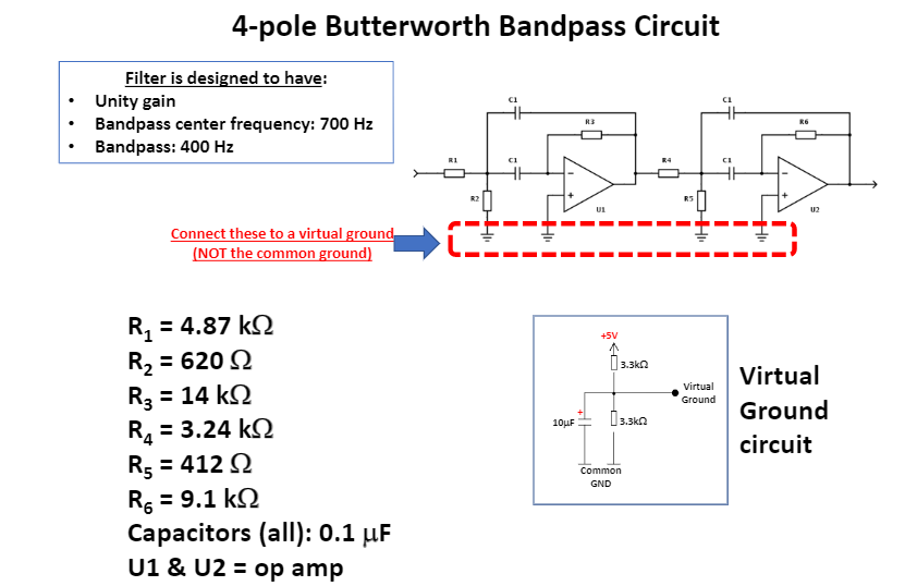
Fig. 11. 4-pole Butterworth bandpass circuit diagram. Image taken from lab handout authored by Carl Poitras.
After modifying the code, we ran the experiment and obtained the following results. Fig. 12 shows the frequency response of the low pass filter, and Fig. 13 shows the frequency response of the high pass filter. We can see that the theorectical and the experimental frequency response barely agree with each other for both of these passive filters. For the low pass filter, the two curves have the same trend above 600 Hz, but we are not able to see further into the spectrum because of the limitation of our sampling frequency. They may agree with each other better if we have higher sampling frequency.

Fig. 12. Frequency response of the low pass filter.
The same conclusion is applicable to the high pass filter. The two curves have the same trend above 600 Hz, but we may also need to use a higher sampling frequency to achieve better agreement between the experiemeental and the theorectical frequency response.

Fig. 13. Frequency response of the high pass filter.
Other factors that may contribute to this inconsistency could be:
In conclusion, we can say that the RC low pass and high pass filter do no perform well in our situation. Therefore, they are not good choices to be used in lab 4.
We then move to the band-pass filter. Surprisingly, the bandpass filter has very good performance! In the bandpass region, the experimental and the theorectical curves agree well enough with each other and has nearly unity gain. Outside of the band pass region, the filter suppresses the frequency response to > -10 dB, which effectively filters out unwanted frequencies from our sound signal. Therefore, the band pass filter is the most practical one out of these three filters: it has the best performance, and it is well-suited for our practical use in lab 4. However, we will still get more confidence on t he band pass filter if we can make our sampling frequency higher and look further into the frequency spectrum. Currently, we cannot see the cut-off frequency for high frequencies outside of the band pass region because of the limitation of our sampling frequency.
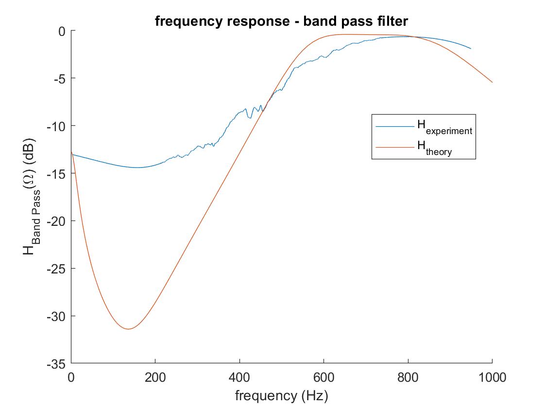
Fig. 14. Frequency response of the band pass filter.
The last step is to put everything together and perform FFT on the Arduino. In this step, we have decided to only use the amplification circuit on the microphone circuit without any filters (also applicable to lab 4) because we have determined that other fellow classmates have many issues with the filters, and it is already sufficient to use the amplification circuit to serve our purpose in lab 4.
In this section, we need to code the Arduino so that it can do FFT on-the-fly versus previous we are doing FFT with MATLAB. In Lab 4, we will use various frequency signals to tell the Arduino to perform certain actions. To perform FFT on the Arduino, we need to write the Arduino program so that in the set-up part, the Arduino will:
In the interrupt service routing for TCA0 interrupt, the Arduino will
What happens now is that after the set up section, the TCA0 sends interrupt signals every 0.41667 ms, meaning that the interrupt service routine will collect one ADC reading value every 0.41667 ms. Then in the loop section, the Arduino will
fft_inputfft_input arrayfft_log_out array which contains the fft results into the serial monitorOnce we understand what tasks are needed to be performed in each step, coding it is just a trivial matter. I coded up a brunch of helper functions in another file and call those functions in the main code section to provide better abstraction. After all, I was able to successfully wrote the code and send the output to the computer serial monitor.
One tricky part is to convert 0.41667 ms to the correct interrupt counter values. This tasks is done in previous labs. I ended up using a interrupt counter value of 6666 with 1X clock divider, which corresponds to approx. 0.417 ms, which I suppose is close enough.
To verify the correctness of my program, I use my phone to play sounds of frequency 500 Hz, 700 Hz, and 900 Hz, used the Arduino to collect data and perform FFT, and copy-pasted the FFT output from the serial monitor to excel for plotting. Fig. 15-17 shows the frequency spectrum from the serial monitor corresponding to 500 Hz, 700 Hz, and 900 Hz, respectively.
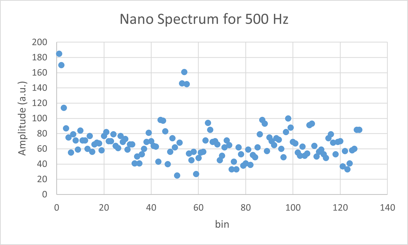
Fig. 15. Frequency spectrum of 500 Hz signal picked up by the Arduino.
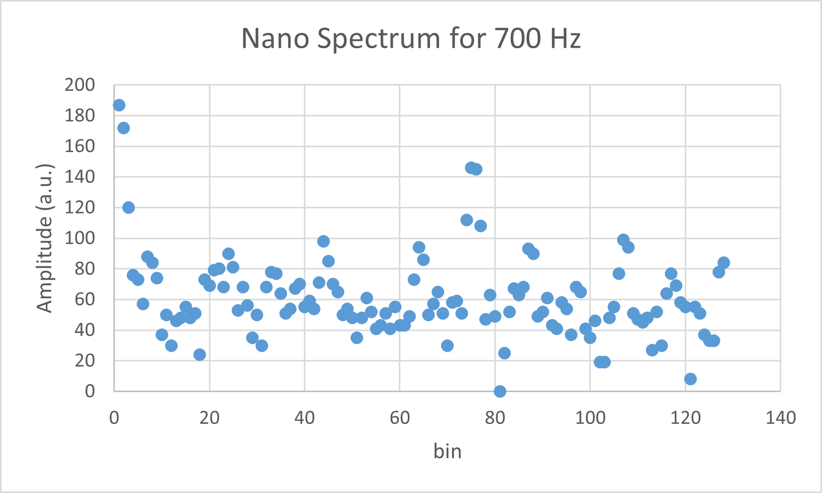
Fig. 16. Frequency spectrum of 700 Hz signal picked up by the Arduino.
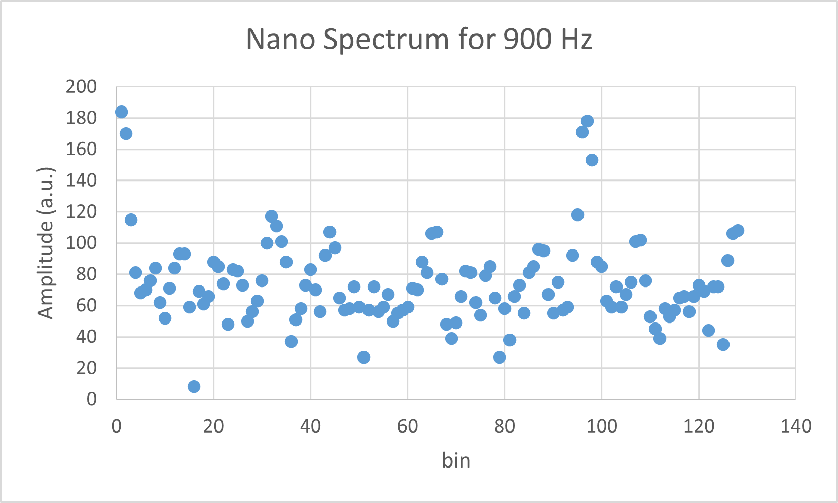
Fig. 17. Frequency spectrum of 900 Hz signal picked up by the Arduino.
Although we did not calculate the frequency spectrum and include that into the plot, we can leverage our knowledge of the Nyquist frequency being 2400 Hz / 2 = 1200 Hz to estimate the position of peaks. We can then conclude that the Arduino is doing the correct FFT as expected from the fact that the 500 Hz, 700 Hz, and 900 Hz signal correspond to peaks in the ~55th, ~75th, and ~95th bins, which is correct considering that we have 128 bins in total. Therefore, our Arduino microphone + FFT combo is ready for lab 4!
In this lab, we accomplished the following tasks:
All these tasks were successfully completed. We built the microphone circuit with the Arduino. We then improved the microphone circuit with an amplifier. We also tested different filters with the microphone circuit to characterize the frequency response, and compare the measurements with theorectical predictions. Finally, we were able to perform FFT on the Arduino to achieve fairely accurate results.
In conclusion, we successfully accomplished all the tasks specified in the lab, and we are ready to take our robot one more step further in lab 4: integrating our previous light-following design to the FFT design and make the robot responsive to frequency signals that we send!