In lab 4 (the last lab!!!), we programmed our Arduino robot to accomplish two demo tasks: an ultrasonic sensing detection robot, and a light-following navigation robot. Specifically, these are the subtasks that we have accomplished (in sequence) in this lab:
This lab 4 report will therefore be organized into 5 main sections, each discussing one of the subtasks above. The Discussion section at the end recaps the goals of this lab.
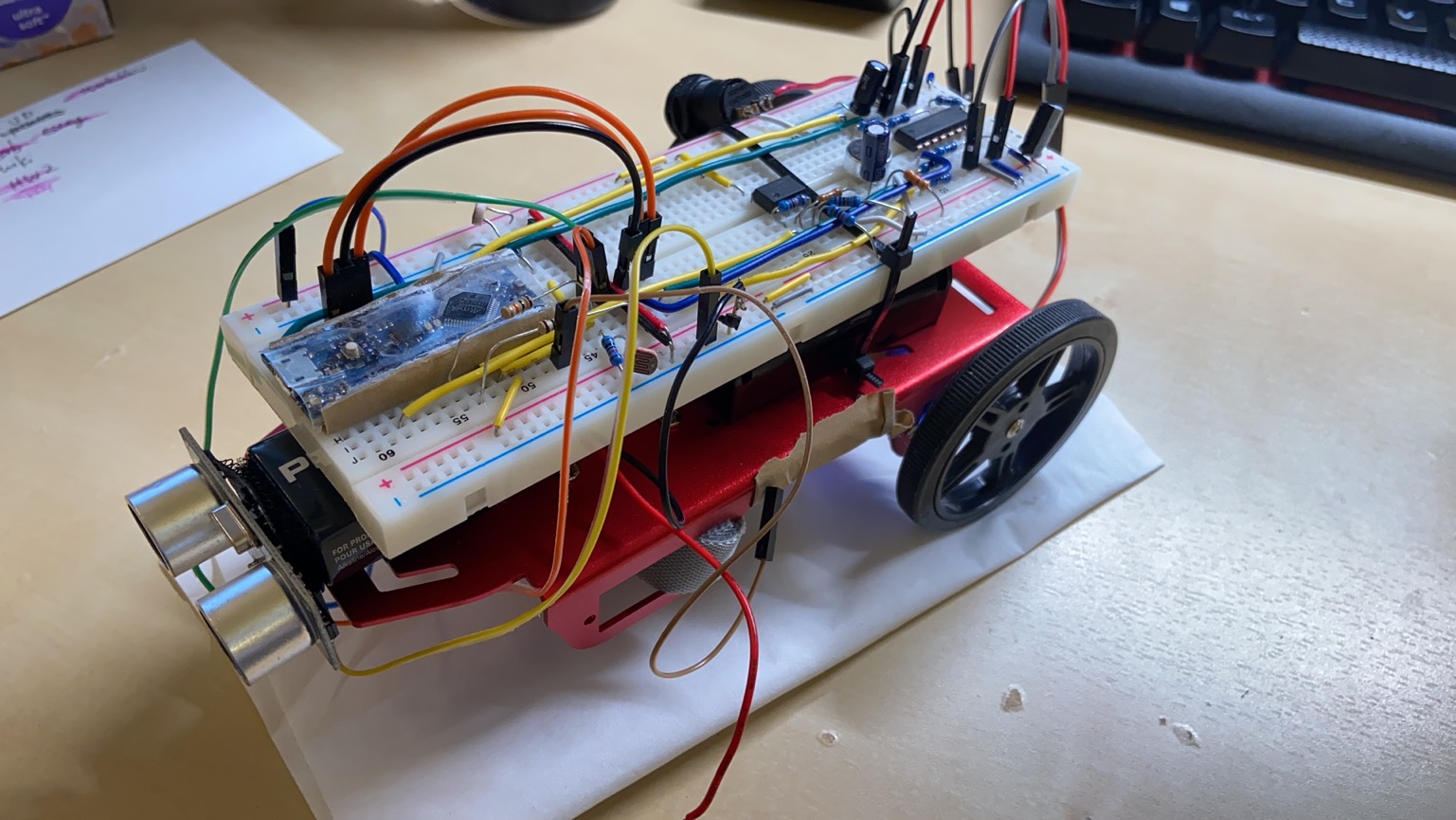
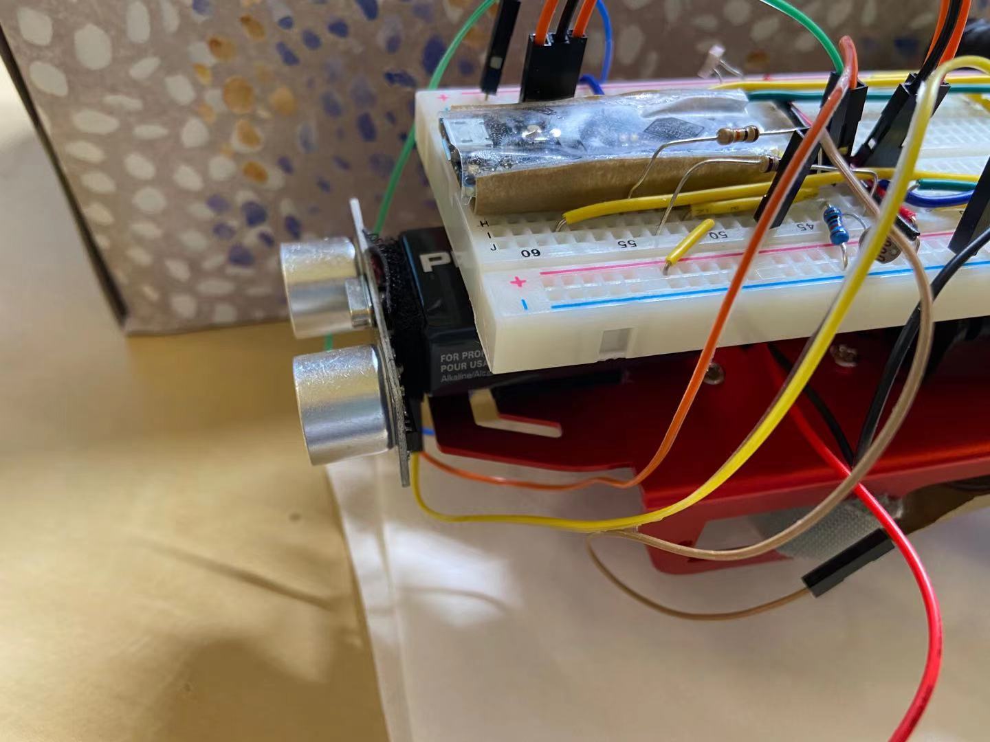
The first step is to physically mount the ultrasonic sensor to the robot. The ultrasonic sensor needs to be on the front of the robot facing forward, so we adjusted the position of the 9V battery and the breadboard to give enough space for the ultrasonic sensor, and we used Velco to affix the ultrasonic sensor to the 9V battery. The figure below shows the physical location of the ultrasonic sensor on the robot.
Because these adjustments moved the center of mass of the robot forward, turns out sometimes the rear wheels that are powered by the motors will be lifted off the ground if the floor is not even. Therefore, we taped a stack of coins to the back of the robot to even out the weight and send the center of mass to the back as shown in the figure below.

The next step is to code the Arduino to use the ultrasonic sensors. This was briefly covered in lectures. There are four pins on the ultrasonic sensor that needs to be connected: VCC, GND, TRIGGER, and ECHO (see figure below). VCC and GND are normal power pins that are connected to the 5V rails. TRIGGER is a digital input PIN, and ECHO is a digital output PIN. Therefore, they will both be connected to one of the Arduino’s digital PINs, and they will be set to digital outpu and digital input on the Arduino, respectively.

The mechanism of ultrasonic sensors are quite basic. When the ultrasonic sensor senses a trigger signal, it will send out eight pulses of ultrasonic sound signal at 40 KHz. It will then set the echo pin to high until it receives the ultrasonic signal that comes back. Therefore, the Arduino will measure the duration of the pulse coming in from the echo pin, and use this time duration along with the speed of sound to calculate the distance to objects. One thing to note is that the ultrasonic sensor should not be triggered so often as the ultrasonic signals could bounce in the environment and create interference, which makes subsequent detections difficult.
An example snippet of code shown in class is as follows (from lecture notes authored by Carl Poitras).
const int triggerPIN = 9;
const int echoPIN = 10;

float soundDuration, distToObjectInCM;

void setup(){
    pinMode(triggerPIN, OUTPUT);
    pinMode(echoPIN, INPUT);
    Serial.begin(9600);
}

void loop(){
    digitalWrite(triggerPIN, LOW);
    delayMicroseconds(2);
    digitalWrite(triggerPIN, HIGH);
    delayMicroseconds(10);
    digitalWrite(triggerPIN, LOW);

    soundDuration = pulseIn(echoPIN, HIGH);
    distToObjectInCM = (soundDuration*.0344)/2;
    Serial.print("distToObjectInCM: ");
    Serial.println(distToObjectInCM);
    delay(100);
}
One could easily reproduce the set up and test out an ultrasonic sensor with this code snippet!
Now that the ultrasonic sensor is hooked up to the Arduino, and the Arduino has a program that uses the ultrasonic sensor, but we still need to make sure the ultrasonic sensor is set up correctly and that it functions well regardless its distance to the object. Therefore, we place an object that is 2, 4, 6, 8, 10, 15, 20, 30, 40, 50 cm away from the ultrasonic sensor, and note down the detected distance from the ultrasonic sensor to make sure it is functioning as expected and the error is low. We then plot a graph of actual distance versus detected distance, superimposed by actual distance versus error, to characterize our ultrasonic sensor setup. The plot can be seen below.

We see from this plot that the performance of the ultrasonic sensor is consistent across all distances from the detected object. The error is higher in very close distance (> 5 CM) but the error becomes negliable when the distance is > 20 CM. Our guess is that the ultrasonic interference is strong when the object is very close to the ultrasonic sensor, thus introducing the errors. However, since we will not detect very close-range objects in our demos in this lab, the error falls fall within the the acceptable regime.
The overall objective for demo 1 is straightforward. The robot starts still with its onboard LED being off. The robot’s initial position are relative to two obstacles as shown in the figure below.
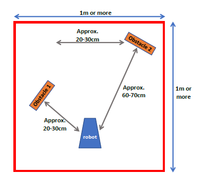
The pilot (that is us) will then play a music that contains a 550 Hz note. As soon as 550 Hz note is played, the robot starts turning. As the robot is turning, it starts detecting the two obstacles. Whenever the robot is facing directly to one of the obstacles, it should detect the obstacle and light up the onboard LED. Whenever it is not facing the obstacles, the LEDs should be off.
This requires the robot to first constantly perform FFT to analyze incoming sound signal. The robot should switch from the “listening” stage to the “turn and detect” stage when it detects the 550 Hz signal. This is done by using a status flag in the program. If the status flag is set to “listen” stage, the “turn and detect” fragment of code should not be executed. On the other hand, if the status flag is set to “turn and detect” stage, the “listening and FFT” fragment of code should not be executed. Once the Arduino detects the 550 Hz frequency (this is done by performing FFT and detect the local maximum from 400 Hz to 700 Hz, and check if the bin that contains 550 Hz is a maximum), it the status flag is switched from the “listening” stage to the “turn and detect” stage, and the robot starts turning.
When the robot is in the “turn and detect” stage, it simply keeps turning and detect objects using the ultrasonic sensors. Of course, there should not be any blocking code, so all the timings involved in the ultrasonic sensor is accomplished by a couple of timing flags similar to the scheme below that was used in lab 2:
void loop()
{
  // execute if reaches status change interval
  if (millis() - status_timer >= status_check_interval){
      status_timer = millis();
      // 1. check lighting conditions
      // 2. modify motor control pins
      // 3. modify LED_enable flag if needed
    }
  }

  // toggle LED_on every 500 ms
  if (millis() - LED_timer >= LED_interval){
    LED_timer = millis(); // reset LED timer
    LED_on = !LED_on; // flip LED_on flag
  }

  // set LED state
  if (millis() - LED_response_timer >= LED_response_time){
    LED_response_timer = millis(); // reset LED response timer

    if (!LED_enable){
      // turn off on-board LED
    }
    else{
      if (LED_on){
        // turn on on-board LED
      }
      else{
        // turn off on-board LED
      }
    }
  }
}
Depending on the distance detected, the robot simply changes the state of the onboard LED. If the distance detected falls within 65 centermeters, then the robot turns on the onboard LED. Otherwise, the robot turns the onboard LED off.
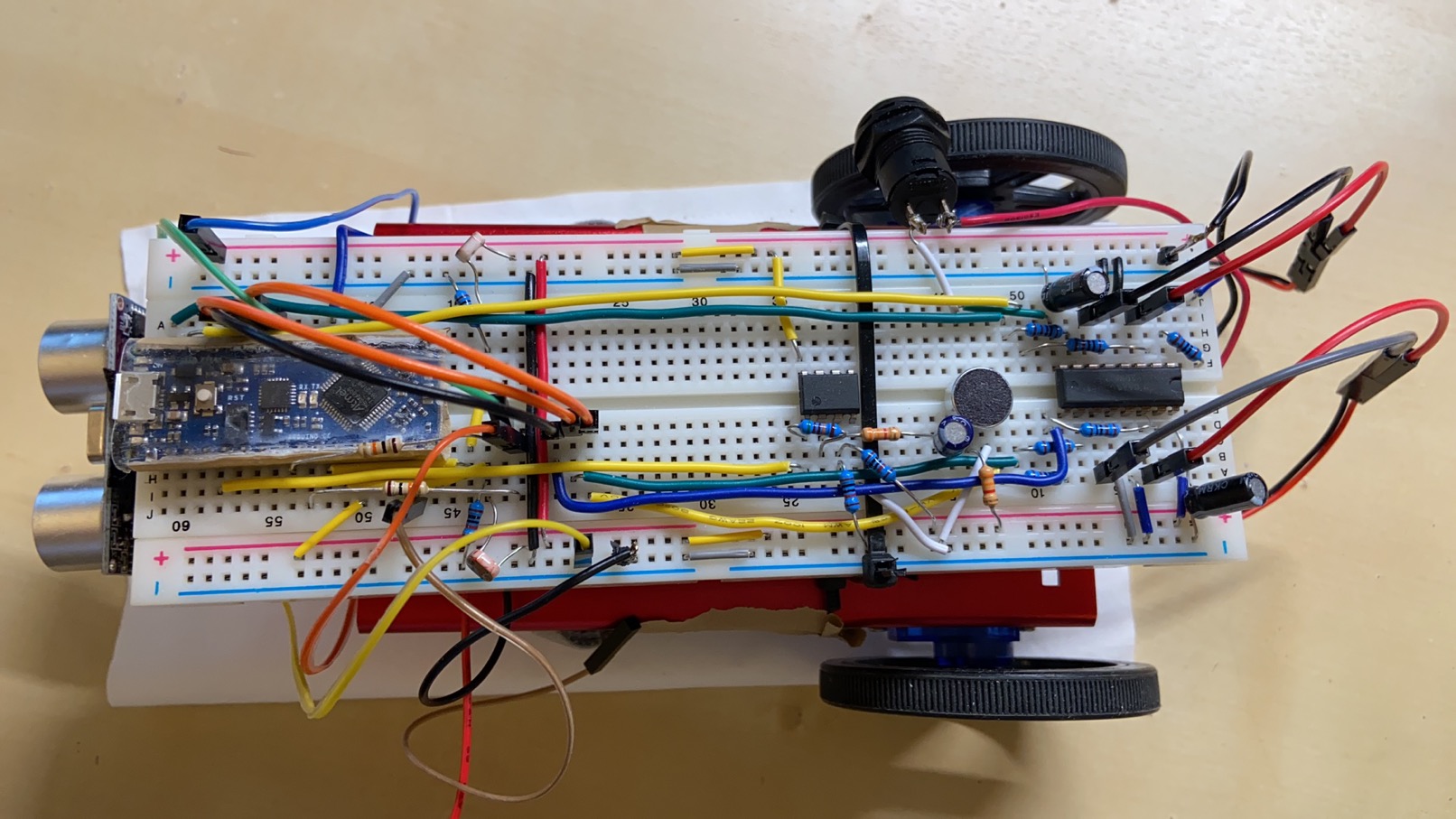
This demo requires the microphone + amplification circuit, the light sensing circuits, the h-bridge and motors, and the ultrasonic circuit. Therefore, we will first need to put everything together on the breadboard so that there are hardware componentts to support the functionality of the Arduino robot. The final breadboard looks like the following:
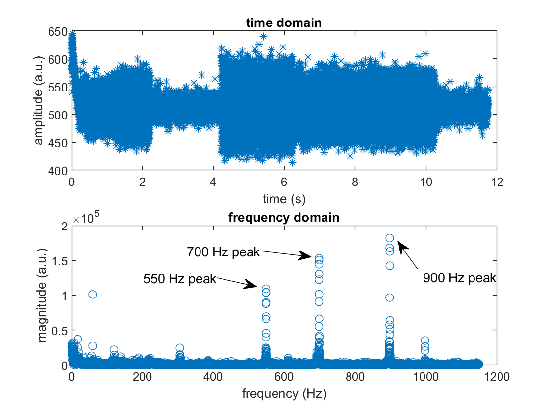
First, we characterized the music file that is played and plot the spectrum of it by sampling sound signal on the Arduino and sending it to the computer MATLAB for FFT and plotting as in lab 3. The figure below shows the time domain and frequency domain signal. We can observe that there are mainly three peaks at 550 Hz, 700 Hz, and 900 Hz. This convinces us that 550 Hz should be the strongest signal from 400 Hz to 700 Hz, and its magnitude will be above a certain threshold. Therefore, we were able to program the Arduino based off of this assumption as it is verified with this FFT test.
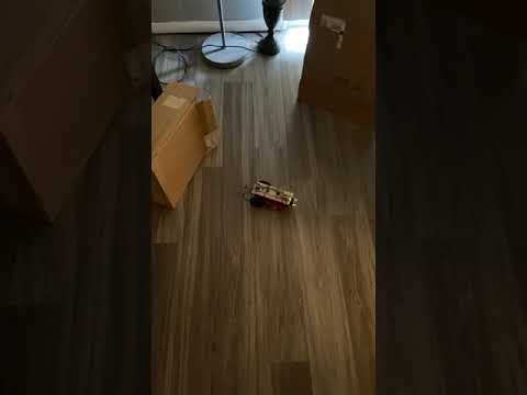
Then we programmed the Arduino with our plan and successfully completed the demo video. The demo video can be found below by clicking the image (it should take you to a YouTube video site). This demo video shows the complete process of me playing a sound, the robot detecting the sound and starts turning, and finally detects the obstacles along the way.
This demo is fairly straightforward and easy once we have figured out the expected behavior of the robot and associate that with some of the programming schemes and subroutines that we have developed over previous labs.
Demo 2 is more complicated than demo 1, the location of the obstacles and the robot moving path is shown in the figure below.
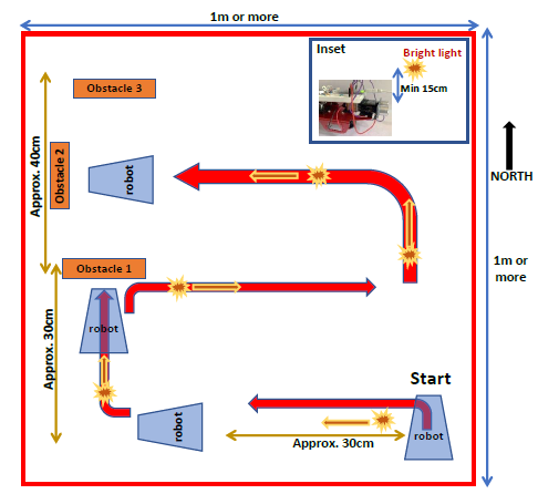
The robot should complete several tasks as described in the lab 4 handout authored by Carl Poitras. I have summarized some of the steps below for reference
This demo is intrinsically more complicated because there are two inputs and two outputs involved.
INPUTS
OUTPUTS
The first thing we can make sure is that we will follow the same programming paradigm, where we will use flags and time intervals to check for time, and we will use various different flags to signal the state of the robot.
There are some patterns that we can observe and take advantage of, which will make programming the robot easier
keep_moving flag. When the keep_moving flag is True, the robot will execute neither the navigation code nor the blocked code. The flag will be reset after keep_moving_interval microseconds.By putting all things together, programming the Arduino is a trivial matter and it only takes time to implement, test, and tune some of the parameters.
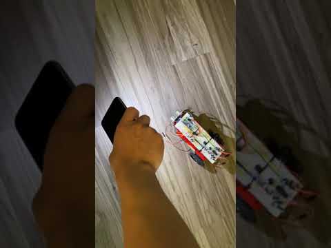
At the end, we were able to take a video of the robot doing what is specified in Demo 2. You can click the image below to view the video. It should take you to a YouTube site where you can watch our demo 2 video. Note that Owen had to use one hand to hold the light source and use another hand to shoot the video so that video quality may not be so perfect. Owen also adjusted the positions of obstacle 2 and obstacle 1 after the robot has collided with obstacle 1 because the robot turns centered in the caster wheel, which could potentially lead to it colliding with obstacle 1 and 2.
In this lab, we accomplished the following tasks:
All these tasks were successfully completed, and we successfully used everything we have built in previous labs including the h-bridge, ultrasonic sensors, light sensors, microphone circuit, etc. Putting everything together was difficult because it requires
At the end of the course, we have learnt about how to use some common microcontroller sensors and actuators, how to build filters, and some programming paradigms that we can use in programming microcontrollers. Though most of the contents are repetitions of ECE 2100, ECE 2200, and ECE 3140, we are glad that we have this opportunity to put everything together and build something ECE!
Final shoutout to our robot!!!