Lab 4

Home Lab 1 Lab 2 Lab 3

Summary of what was accomplished during the lab

• We soldered the RF transmitter and receiver together
• We wrote the code for the base station RF receiver and RF transmitter for the robot and tested it
• We merged all parts of our code together for the robot including FFT, reading the light frequency from the photo transistor, servo motor control, and RF transmission
• We merged all parts of our code together for the base station including the 7-segment display and RF receiver
• We wrote a movement algorithm for our robot
• We wrote a navigation algorithm for our robot
• We wrote an algorithm to determine if we have seen two treasures
• We updated the FFT to check if we had heard a 950 hertz signal
• We added the state logic for the entire demo
• We got rid we got rid of all delays and analog read usage in our code
• We thoroughly tested our robot

RF Transmitter and Receiver Assembly and Testing

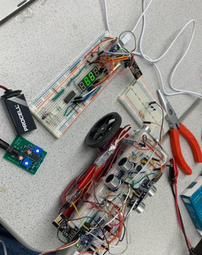
We first soldered the RF transmitter and RF receiver after confirming that our pins were in the correct places. Then we edited the RF code for the transmitter and receiver so that it would be using the correct pipes. Then we tested it and found that the robot and base stations were able to connect and send data over.

Here is a picture of our RF setup:

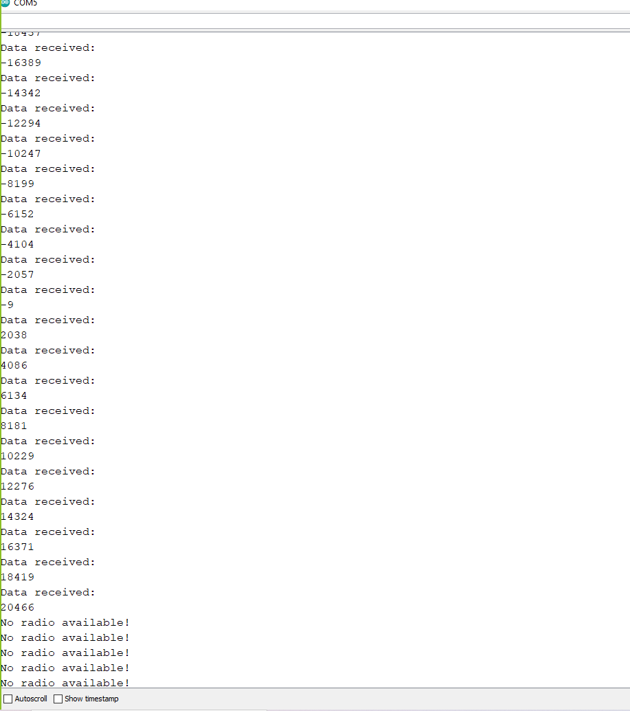
Here is a picture of our RF data being sent:

Merging code for the Robot

We started by having one file for all the code, but then we split it up into a file for the FFT, US sensor, servo control, navigation, IR frequency detection, RF, and main runner file for all our code. We brought each part of the code over and created setup functions for each of them that would be run inside the main setup function and then confirmed there are no delays or other commands that were not allowed in the code. Following this, we create test functions for each functionality, like reading the ultrasonic sensor values come and used these types of functions to test each part of each merged code individually, and then together to confirm there are no problems with the code affecting each other. We found there were several cases of the code breaking other parts of the code, like SPI from RF when you wanted to blink the LED or interrupts with the FFT messing with other parts of the code. We made the required changes, like using SPI.end() and not using sei() and cli() to stop the FFT interrupts.

Merging code for the Base Station

We began by separating the RF code and a 7-segment code into two different files and then had the 7-segment code call the RF code as needed to get new data received as well as a setup function for the RF code. This was then tested and validated with the robot to make sure frequencies being sent from the robot values via RF could be received. We also updated our RF code to version two.

Writing a Movement Algorithm

Our, movement algorithm consisted of having series of commands that allowed for us to move based on our position. So whatever command the navigation system wanted to run, it would run it, and then the movement algorithm would run it until completion of the movement, where we it would then set a flag and allow for the robot to scan its surroundings and decide what to do based on the navigation algorithm. We were able to turn, turn with timings, and turn using sensor data by comparing the front sensor value to the side sensor value and saying a turn was complete when the side sensor value matched that of the previous front sensor value that was recorded before the turn started. We could also move forward and backwards with non-blocking delays by using timers.

We also made it so that the forward control system was a bang bang controller, where if the US sensors tell us that we are closer to the left wall, then we would turn right with a set value. If we were closer to the right wall, then we would turn to the left with a set value. In the case that we were within a "dead zone," meaning the value too small to be considered, we would just drive forward with no turning.

While using our bang bang controller, it was possible to drive past an empty wall and swerve by accident. To avoid this, we saved the previous us value and used it if there seemed to not be a wall next to the robot so that we would not swerve.

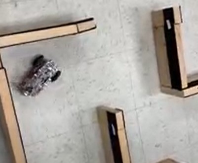
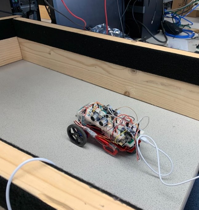
Here is a picture of us turning during the final competition:

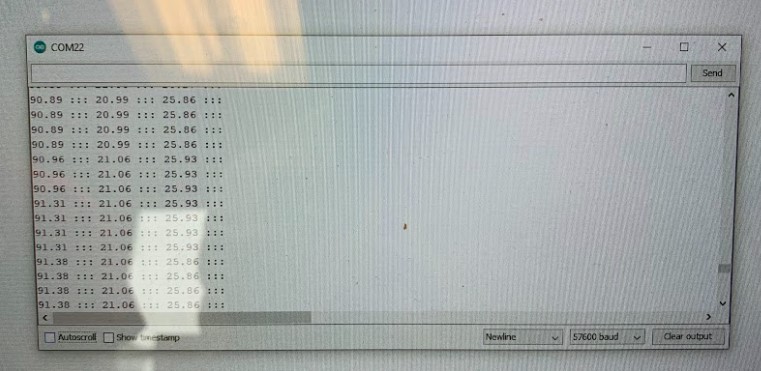
Here is a picture of the serial monitor when testing our US sensors during the final competition:

Writing a Navigation Algorithm

The navigation algorithm was initially using depth first search. We would first see if it was possible to move forward. If it was not, if it was possible to move to the right. And again if not, if it was possible to move to the left. If all these options were not possible, then we would backtrack to our previously unexplored position. We had a way for us to keep track of our heading, a way to both build and use a map of the maze and determine where we had visited and keep track of how far we had moved based on the sensor readings of us moving forward.
We unfortunately had to scrap these algorithms due to hardware constraints and instead used the right wall follow algorithm that would follow the right-hand wall as we drove around and would also make sure that we would not get stuck on right turns, meaning if we if we had just turned right we would drive a little bit further forward to ensure that we would not just turn right again.

Here is a picture of our US and navigation testing:

Treasure Finding Algorithm

Our treasure finding algorithm first started with the frequency detection system. We would only detect the frequency between 1000 and 10000 hertz and when we detected a frequency between that range, we would check that we got 5 values in a row with similar magnitudes. If we did, this meant we had likely found the treasure and so we saved that as a treasure frequency and sent it to the RF transmitter to be sent to the base station. Then we would again search for another frequency, and we would have to be a certain percentage different than the first treasure frequency and then we would save it as a second frequency and send it to the base station. Once the second frequency was found we would raise a flag telling the system both treasures were found. This flag would stop the robot and make the LED blink.

FFT 950 Hz detection algorithm

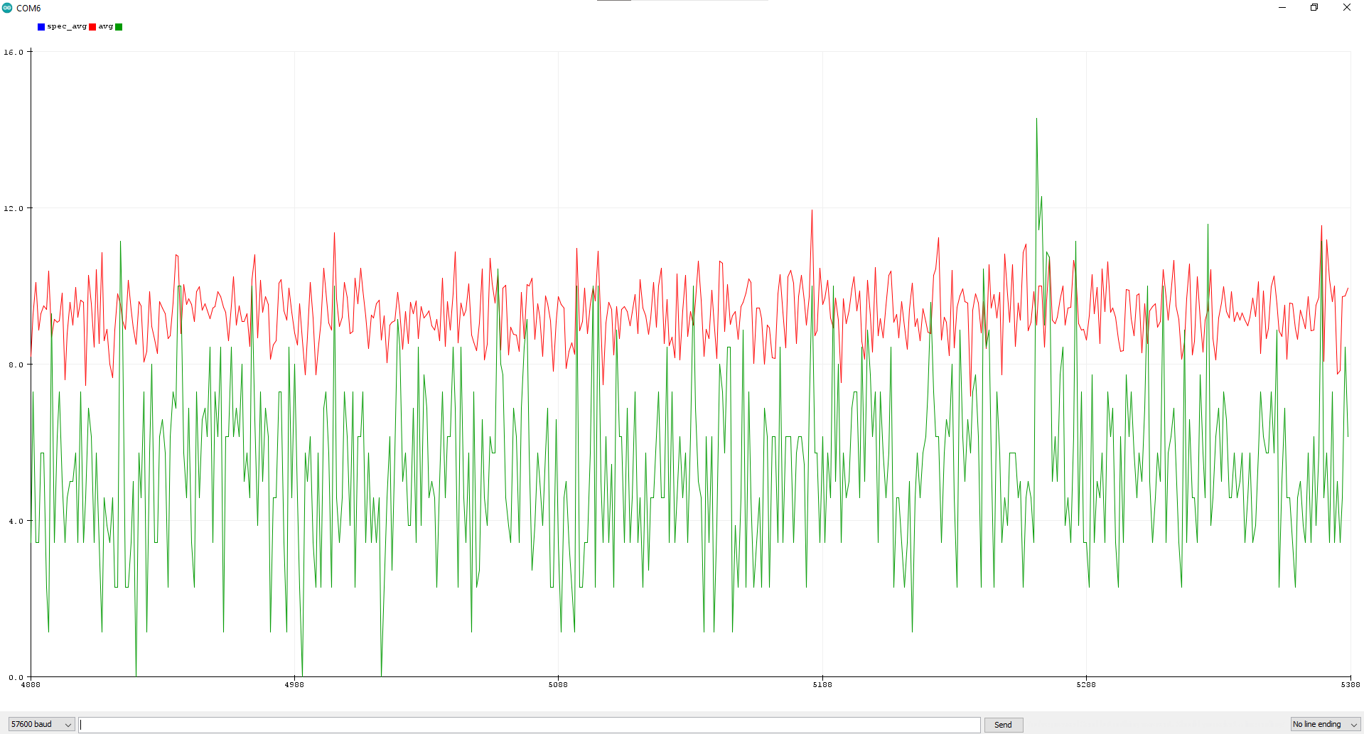
We used the FFT code from lab 3 and had it loop until it found the 950 Hz frequency. We detected the frequency by averaging the last 97 bins and then comparing this to the average of the 6 bins around the 950 Hz frequency bin and the 950 Hz frequency bin. If this 950-bin average was large enough, then the frequency was found and we exited the loop, otherwise, it would reset the FFT for another detection cycle and then run it again.

Here is a picture of us comparing the 950 and side bin averages (bottom graph) to the average sound frequencies from 30 to 127 (top graph).

State Logic for the Demo

Our logic for the demo first started with the setup for each sensor and movement component running. Then we sent a handshake to the base station of 8888 to ensure a connection was made. Then we would start looking for the FFT frequency of 950 hertz. If we found it or if the button was pressed, the robot would move on to the next state and send 7 to the base station to make sure we were still connected. Following this, we ran the navigation algorithm and navigated around the maze finding treasures until we found two treasures. Once two treasures were found, we would set a flag to tell the code that two treasures had been found and then we would enter the end state where we would stop and blink our led.

Cleaning the Code

For cleaning the code, we made sure no delays were used, except for delay microseconds, and no blocking commands were used.

Here a picture of our assembled robot with the base station

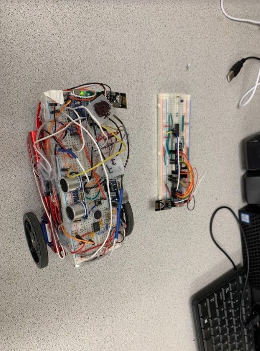
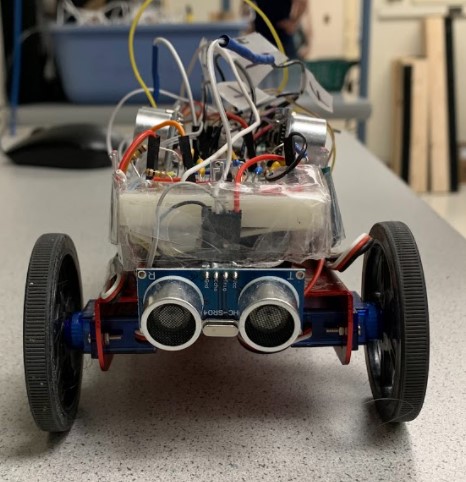
Here are some other angles of our robot. The black wires were used to have a better connection with the breadboard by stripping a longer piece of wire since we were having connection issues. They were labeled F, R, and L for front, right, and left US sensors and again F, R with a black dot, and L with an I for the front, right, and left IR sensors:
Front of Robot:

Left of Robot:

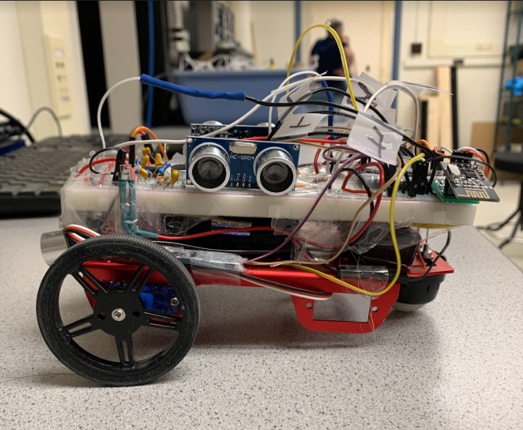
Right of Robot:

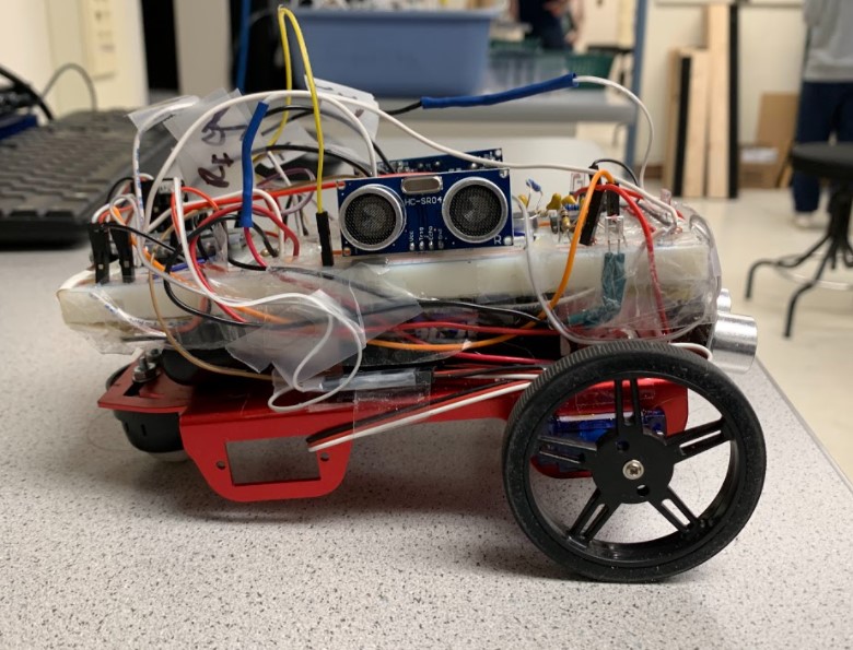
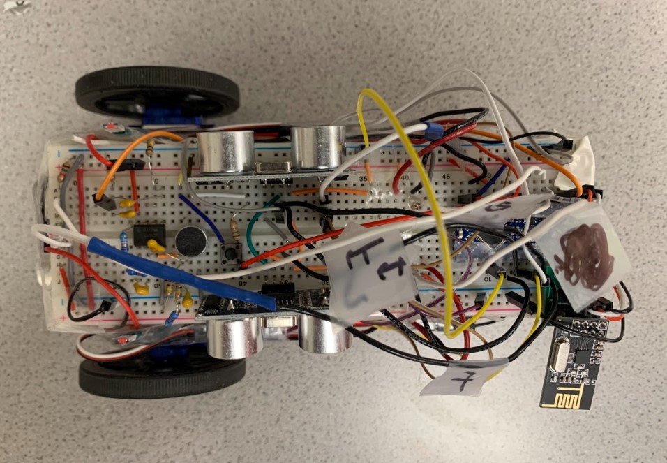
Top of Robot:

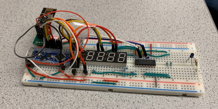
Here are some pictures of our base station:
Front of Base Station:

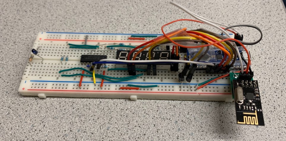
Front of Base Station:

Here is a video of our demo, sped up and compressed to fit in GitHub: