Lab 2: Analog Circuitry and FFT’s

For this lab, we divided our team into two subgroups: An Acoustic team and an Optical/Treasure team

Acoustic Subteam

• Trisha
  
• Jimmy
  
• Yonghun
  

For this section, we used the following materials:

Software:

• Arduino IDE (Available Here)
  

Hardware:

• 1 Arduino Uno
  
• 1 Electret microphone
  
• 1 (1 µF) capacitor
  
• 1 300 Ω resistors (measured value of 327 Ω)
  
• 1 3 kΩ resistor (measured value of 3.27 kΩ)
  

We first installed the Open Music Labs FFT Library onto Trisha’s computer, as she was the one actually writing the code for this lab. You can download it here

We looked at the fft_adc_serial file example, which collects data from A0, performs the fft, and then prints to the serial monitor.

Yonghun setup the signal generator with a 660 Hz and 1 Vpp, .5 V offset signal. We decided we would rather use the signal generator at first so that we could be sure that the program was working as expected before we implemented the tone generator on a phone. We checked to make sure the signal generator was working on the oscilloscope.

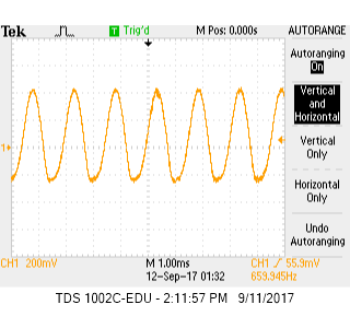
As shown in the screen capture above , the signal from the sine generator acted as we expected.

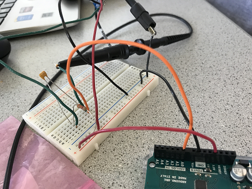
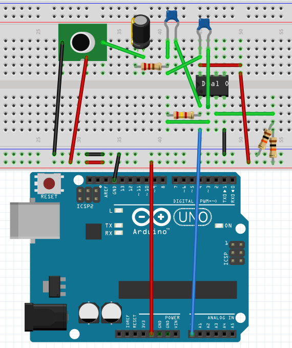
This was our circuit with the oscilloscope hooked up. We ran our output into the A0 analog input port on our Uno and fed the circuit 3.3 V.

After getting the Open Music FFT Library installed, we opened up the example fft_adc_serial and began to look through the code and test it out. We we checked the serial output to see what the program was reading we ran into an issue. The output was a bunch of random symbols and gibberish that meant nothing. We double checked the signal generator to make sure it was still working and it was.

We debugged the code and found that the serial monitor was running on a different frequency than our board, so we switched the baud frequencies to match. Then we started getting actual data.

Although we started getting data we didn’t actually see our 660 Hz peak anywhere. We realized that our scale was wrong so we recalculated it. We kept the prescaler at 0xe5, which was the 32 division factor. That means that the bin width is 150 Hz. 16 MHz / 32 division factor / 13 clock cycles = ~38 kHz. Divide this by the 256 samples, gives you 150 Hz/bin. Once updated in our data sheet it gave us the correct peak on our frequency graph.

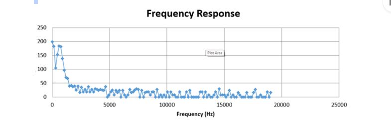
We placed all of the outputs into an excel table and used the bin width to graph this frequency response. The two points on the peak are 600 Hz and 750 Hz so our 660 Hz peak is shown.

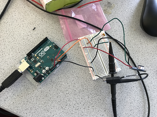
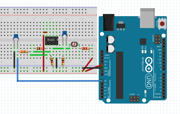
Once we got the code and excel working, we added the microphone into our circuit and began data collection using the oscilloscope to get a feel for the frequencies we heard.

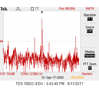
Shown above is the oscilloscope screen capture of the microphone hearing the 660 Hz tone. The oscilloscope was calibrated to 660 Hz so the spike in the middle of the screen represents the 660 Hz tone, the rest is noise.

We also tried to incorporate an op amp that had the following circuit:

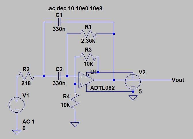
We decided whether or not to use a an op amp as an active filter by taking data from close and far with the op amp and without it and compared. Our op amp has a 30 dB gain and the circuit is tuned for roughly 660 Hz.

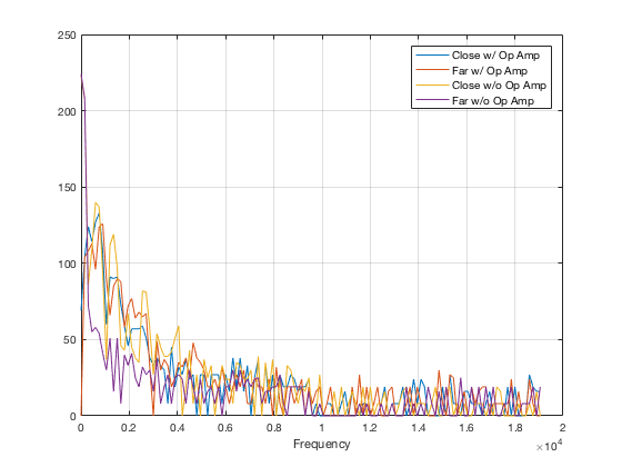
This graph gives a summary of four different test cases. We wanted to test using the op amp versus without it as well as what the microphone could pick up when the Tone Generator was close to it versus far away. To take a closer look at this data, we graphed the data using MATLAB to only compare the data with or without using the Op Amp.

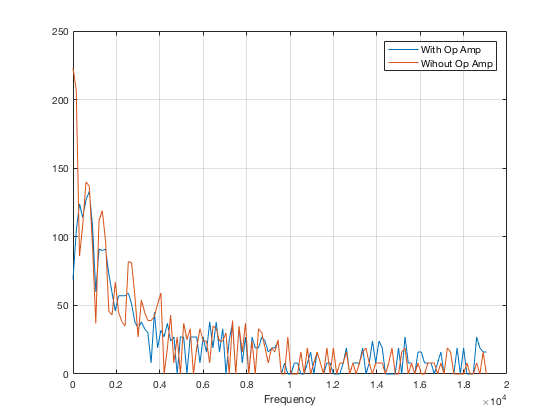
As you can see the op amp got rid of some of the noise which would make it easier to locate the 660 Hz signal.

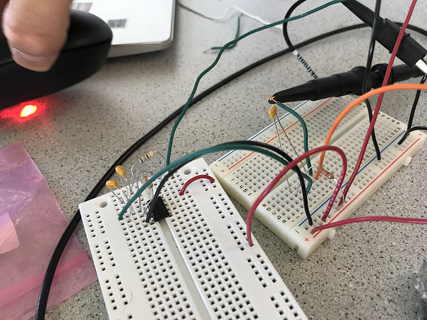
Above is our completed circuit with the op ap

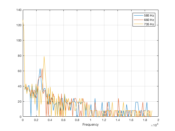
Lastly, we wanted to test to see if we were able to detect different frequencies. Graphing our data, we concluded that we were able to achieve this if we changed our code to analogread().

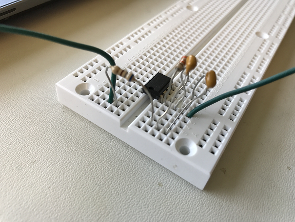
This is a close up of our op amp we used

Optical/Treasure Subteam

• Francis
  
• Paige
  
• Logan
  

For this section, we used the following materials:
Software:

• Arduino IDE (Available Here)
  

Hardware:

• 1 Arduino Uno
  
• 1 USB A/B cable
  
• 1 Phototransistor
  
• 1 330 Ohm resistor
  
• 1 2.2 kOhm resistor
  
• 1 Treasure
  

Like the Acoustic subteam, we first started by downloading the Open Music FFT library and hooking up a basic circuit with a function generator in series with the 330Ω resistor to check the output of the fft_adc_serial example program. We checked the output when we drove the circuit with a sine wave at 7kHz, 12kHz, and 17kHz, 1Vpp and 2.5V offset. We originally tried driving with no DC offset on the function generator and could not distinguish any peaks. This was not an issue, however, when we added a DC offset nor was it an issue later when detecting IR treasures. We collected the data from the serial output and graphed the data in Google charts to get the following graph.

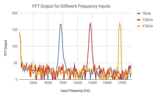
We used the same algorithm as the Acoustic Team for calculating a bin width of approximately 150Hz. With this in mind, we predicted and then verified from our data the bins for the different frequencies, as shown below:
| 7kHz | bin 47 |
| 12kHz | bin 80 |
| 17KHz | bin 114|

By looking in these bins, we can clearly distinguish when we detect a treasure and which frequency by thresholding the values above a certain number we are unlikely to find noise, like 50 for example.

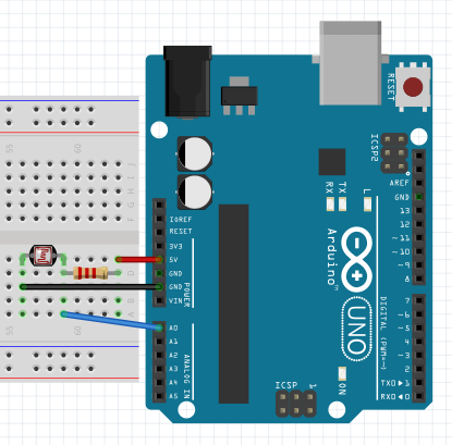
We then set up the IR circuit with the phototransistor (below) and tested its ability to detect the treasures at the same frequencies when placing the treasure board approximately 2 inches away. (See note at end on how to use treasures.)

These are the results we got:

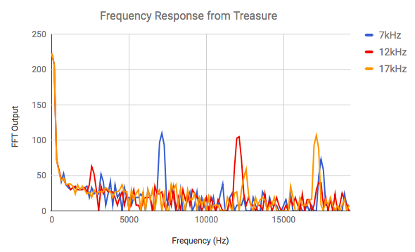
While the peaks are smaller than when produced with a function generator, we can still clearly see and distinguish between the different frequencies of the treasures.

We then wanted to test how the filter would function with outside interference, so we redid the same test with the IR sensor next to a window so that it would also be detecting sunlight.

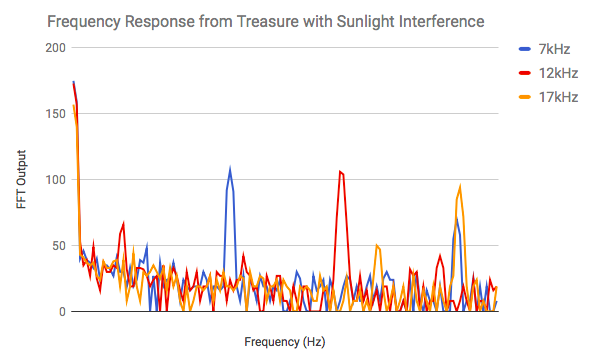
It appears as though there may be a little bit more noise in this scenario, but we still have a very good signal-to-noise-ratio (SNR) and the peaks for the necessary frequencies are still easily distinguishable. Our only concern is that the 7kHz signal seems to be producing a substantial peak at 17kHz as well, both in this case and the one without sunlight. Our code for distinguishing between the two frequencies will have to reflect this.

We also tried to implement an analog bandpass filter to see if we could cancel some of the noise at the lower and higher frequencies we don’t care about.

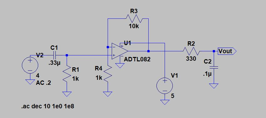
For a 7kHz IR signal, we got the following results.

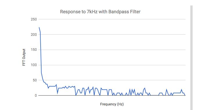
Clearly, the filter not only filtered out high and low filters, but also filtered out the desired components as well. Interestingly, however, there is still a very strong DC component that we do not seem to be able to filter out.

Using Treasure:

The treasure looks like the following

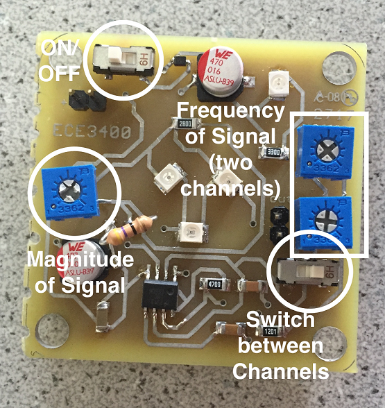
To turn it on, switch the on/off switch. An LED will turn on to indicate that it is on. Turning the magnitude and frequency dials will change the magnitude and frequency of the IR signal. You can store up to two frequencies on the board and switch between them with the switch in the bottom right corner.

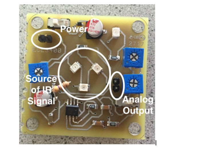
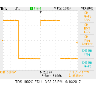
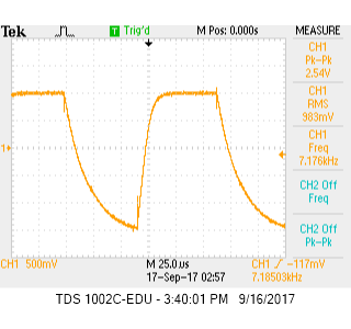
If there is no battery, connect the power pins to a voltage source at 3V. In order to determine the frequency of the output signal, connect the analog output pins to an oscilloscope. The orientation of the pins (flipping +/-) will look differently on the oscilloscope screen, but the frequency is the same for either. It will look like either of the two:

The three squares in the middle are the components responsible for sending out the IR signal, so be sure that the phototransistor can see them. We also found that the orientation of the phototransistor can determine whether or not it can detect a signal. Make sure the wider side of the phototransistor is parallel to the board in order to pick up data from the treasure.

Other Notes

About FFT Library:

After looking at the fft functions from the Open Music website (linked Here) we noted the following things:

There are two pre-processor functions that must run before running the main fft_run() function:

1. fft_reorder()
   
2. fft_window()
   

The main function, fft_run(), assumes that all the data it needs is stored in the array fft_input with the real part of the signal at even number values and the imaginary part at odd number values. For example,

• fft_input[0] = real1, fft_input[1] = imaginary1
  
• fft_input[2] = real2, fft_input[3] = imaginary2
  

The output of fft_run is placed in fft_input in the same organization. Therefore, for a 512 array, there are 256 data points.

About ADC:

After looking at the data sheet for the ATMega328 processor ((Available Here)
we noted the following things:

• The adc takes 25 clock cycles to turn on
  
• ADMUX register determines which analog pin to take data from
  
• ADCSRA determines the scaling factor for dividing the sampling frequency. For example if this register is given a value of 5, the sampling frequency is
  (processor speed)/(2^5)/(13 clock cycles to complete) = 16MHz/(2^5)/13 = 38kHz.
  

Common issues:

• Can’t find file/library:
  try moving the file up a directory. For example, we had several issues getting the compiler to recognize the FFT library; following the directions on the Open Music FFT site, we placed this file in /Users//Documents/Arduino/Libraries/. Move the FFT file up a directory so it is in the same file as Libraries, i.e. you should have /Users//Documents/Arduino/FFT/.
  

• Serial giving gibberish:
  make sure the baud rate selected for serial monitor is the same as the baud rate specified in your code. For example, if you have Serial.begin(9600), you are asking the board to print to the serial at a frequency of 9.6kHz, so the serial monitor baud rate should be receiving at the same rate. You can locate this rate in the bottom right corner of the serial monitor.