Go To:
Home Page

Milestone 4: Maze and Treasure Mapping

Spacebrew Yonghunz

Goals:

For this milestone, we needed to:

Successfully display walls and treasure on the screen as the robot finds them
Signal that the robot has completed the maze via audio and on the screen

Communication Pipeline

Team members:

Jimmy, Trisha, Paige

Materials Used:

FPGA
2 Arduinos
VGA connector and monitor

SPI

In order to communicate location, treasure, and wall information from our robot (Calvin) to the screen, we needed to finalize our communication protocols. The wireless portion was already complete, but communication between the Basestation Arduino and the FPGA as well as between the FPGA and the screen required more work.

Our communication between the basestation and the FPGA is achieved via SPI protocol. It works by taking in 3 inputs: MOSI, SCLK, and Slave Select (SS). MOSI represents the actual data being transferred, SCLK is the clock frequency we are communicating with the arduino at, and Slave Select is the signal that tells us that the arduino is sending data. SS is high the entire time a message is being sent and goes low at the end of it. At the posedge of SCLK we check to see if vgaCS is high and if it is, we bitshift the MOSI bit into a variable to start to build a message that we will later decode. If vgaCS is low, we simply ignore the MOSI bit. Also, we set the other SS pin for radio communication HIGH to unselect that slave during the SPI communication between the arduino and FPGA. You can see this in the following code:

  digitalWrite(10,HIGH);  //unselects radio MOSI
  digitalWrite(vgaCS,HIGH);   //tells FPGA to read
  SPI.beginTransaction(SPISettings(1000000,MSBFIRST,SPI_MODE0));
  SPI.transfer16(got_message);
  SPI.endTransaction();
  digitalWrite(10,LOW);
  digitalWrite(vgaCS,LOW);

At the posedge of CLK, the 25 MHz clock of our FPGA which is much faster than SCLK, we check to see if SS just went from high to low, which represents the end of a message. To do this comparison we save the current SS value into a previous variable at the end of each loop so we are constantly comparing the new SS value to the previous one. If it did just drop from high to low, we know that we can dissect the message into the specified bits to get the information we need from it. This is the breakdown of each bit in the message:

X1, X0 = X location
Y2, Y1, Y0 = Y location
W3, W2, W1, W0 = walls
T1, T0 = treasure
Done = done signal

These bits gets sent as outputs to DE0_NANO which then uses them to update the screen.

To test the SPI was working we tested it in three incremental steps. First we made a module that takes the place of our SPI_COMMUNICATION module and sends hardcoded values into the DE0_NANO to see if our display updating code worked correctly. This test ran through 4 random locations, two of those treasures, and had walls arbitrarily placed. This is that test in action:

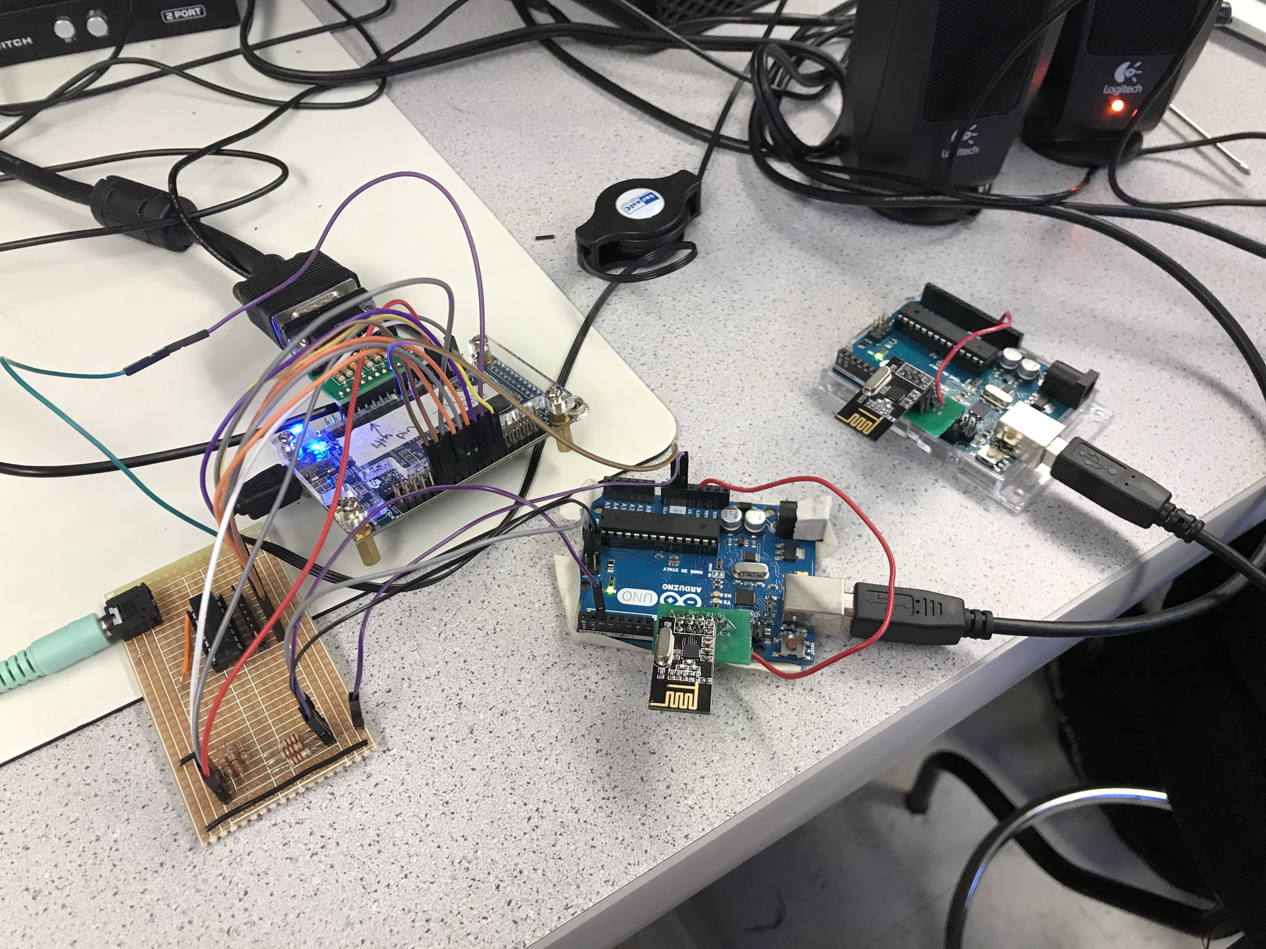
Next we send hardcoded values from the base station arduino through the SPI to see if our SPI could breakdown messages correctly. Instead of sending the got_message from the radio through the SPI, we hardcoded a value such as unsigned int test2 = 1156 which corresponds to 0000010010000100 in binary. Then we probed the SCLK and MOSI line with the oscilloscope to make sure we got the right values. This tested the full base station system and once we felt confident our SPI could breakdown the message correctly we moved onto testing the full communication system. This entailed sending a message from an arduino on our robot, that message being received by our base station arduino, then being passed through our SPI to the FPGA which correctly updated the screen. Here is a video of that test running:

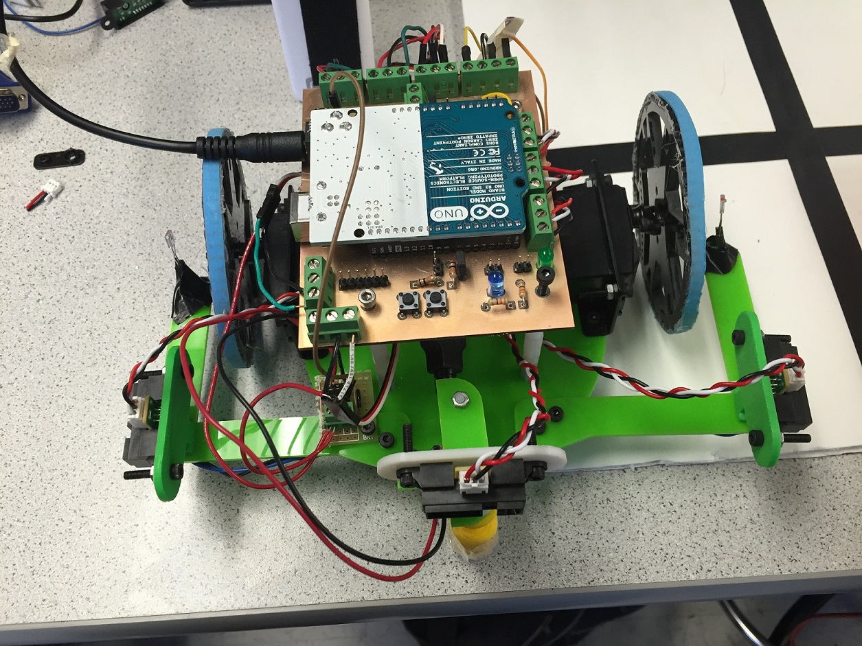
Here is a photo of our full system setup:

On the left is a perfboard that runs our digital output for playing the tune through a DAC which then sends that to an audio jack which plays it through the speakers in the top right of the photo. The FPGA is the component to the right of that which is connected to a VGA display switch. You can see the 8 digital output pins running to the PCB. To the right of that is our base station arduino, which has MOSI, Slave Select, and SCLK connected to the FPGA. Finally, all the way to the right is the Sender Arduino, which sends the data from the robot to the base station arduino.

In order to simulate the robot going through the maze, on the receiver side code for the radio signal, we hard-coded values for the x position, y position, walls, treasures, and done using an array as seen here:

int index=0;
int wallArray[] = {10,10,10,12,5,5,6,10,10,11};
int yArray[] = {0,0,0,0,1,2,3,3,3,3};
int xArray[] = {0,1,2,3,3,3,3,2,1,0};
int treasureArray[] = {0,0,0,0,1,0,0,0,3,2};

Then we iterated through each array with the following code, incrementing index after setting the value of message:

while(index==10);
  message = 0; 
  return_message = 0; 
  walls = wallArray[index];
  x = xArray[index]; 
  y = yArray[index];  
  treasure =treasureArray[index];
  if(index==9){
    done=1;
  }
  else{
    done = 0;
  }

//to update new location of robot
//putting numbers to appropriate bits
  x = x << 9; 
  y = y << 6;
  walls = walls << 2; 
  treasure = treasure;
  done = done << 11; 
  message = x + y + walls + treasure + done; 
  index = index+1;

Note: We had to add a reset button so that we can reset our done signal, x and y values, treasure, and wall values in between tests

Wall

We broke down our VGA display into a 4 by 5 grid representing the locations in the maze. We had to decide how we wanted to implement the walls based off this. We narrowed it down to two options: one being that the walls could become part of the grid and the other being each grid location could be drawn to have the specified walls instead of just a color. We finally decided that it would be much easier to just add the walls into our grid. Breaking down our display to account for these walls took much longer than we thought as it was extremely tedious to figure out how many pixels each wall would be. This pixel distribution was done in a module we named Memory_grid that broke down the display. We thought it would be much easier to do this outside of our DE0_NANO. After a lot of debugging we got it all sorted out and came up with this scheme for interacting with the walls:

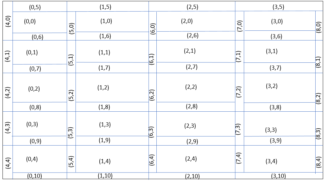
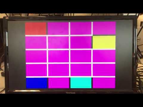
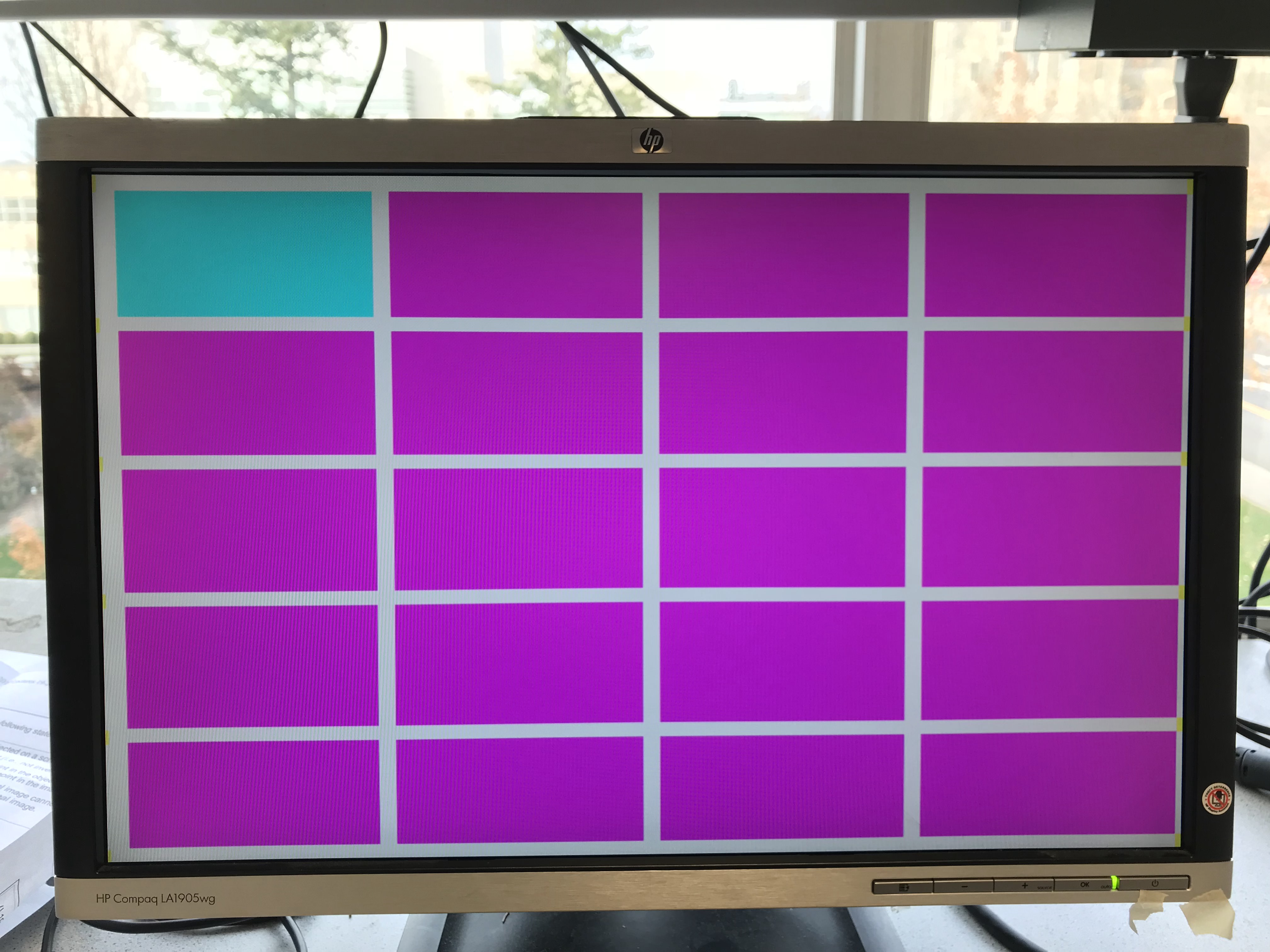
To set up the display we had to initialize everything to the correct color to start it. All of the grid locations were defaulted to magenta, which is the color we decided on for an untraveled location. All of the walls around the outside of the maze were defaulted to black, the color of a wall. All of the potential wall locations inside the maze were defaulted to white, which represents where a wall could possibly be (but we haven’t detected one there yet). We originally had the walls blending into the grid location next to them but it was buggy because there was a lot to check to make sure it matched and depending on where the robot was the walls would change which grid they blended into. This ended up looking very sloppy so we decided to just have all the walls locations visible from the start and update them as needed. When everything was done being set up our display looked like this:

Updating the grid
The next challenge with the VGA display was taking the information the SPI received and using that to update the screen. We decided to add a reset button to make testing it easier and ended up putting the initialization code mentioned before into that part. Next we had to check to see if our previous locations were different than our current locations being received from the spi. If that was true then we knew that the location had changed and we should update the grid.

To update the grid we first had to deal with our previous location we first had to make sure that the previous location was not a treasure. If it was then we simply left it as the specified color to match the frequency treasure in that location. If it was not then we updated the grid location to be yellow, which represented a traveled to location.

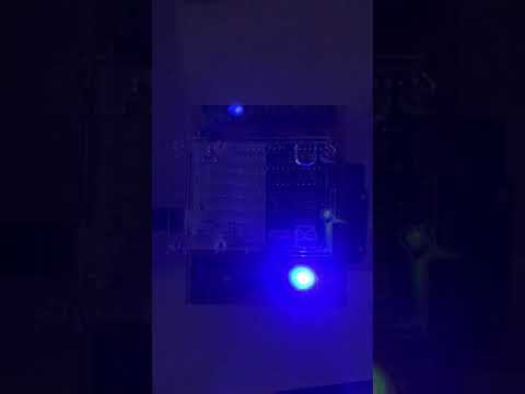
After updating previous location, we then turned our attention to current location. Current locations color was specified by the treasure information. 2’b00 represented no treasure and then the location was set to teal, representing the current location of the robot. 2’b01 represented the 7 kHz treasure and the location was set to red, 2’b10 represented the 12 kHz treasure and was set to green, and finally 2’b11 represented the 17 kHz treasure and was set to blue.

The last part of updating the display was updating the walls. Because we chose to have the walls in our grid this task was fairly easy. Our wall information was 4 bits: [ X3 X2 X1 X0 ]. X3 represented the wall true north of the location, X2 represented the wall true east of the location, X1 represented the wall true south of the location, and lastly, X0 represented the wall true west of the location. This code snippet is everything we had for updating the walls, you can see how easy it was as we simply looked at each bit of wall then turned the specified wall black or left it white:

==================================================================
if(wall[0] == 1'b1) begin
	grid_color[X_CURR+4][Y_CURR] = black;	//West Wall
end
			
if(wall[1] == 1'b1) begin
	grid_color[X_CURR][Y_CURR+6] = black;	//South Wall
end
			
if(wall[2] == 1'b1) begin
	grid_color[X_CURR+5][Y_CURR] = black;	//East Wall
end
			
if(wall[3] == 1'b1) begin
	grid_color[X_CURR][Y_CURR+5] = black;	//North Wall
end
===================================================================

Before we moved on we set X_PREV = X_CURR and Y_PREV = Y_CURR so that we could check for the next movement.

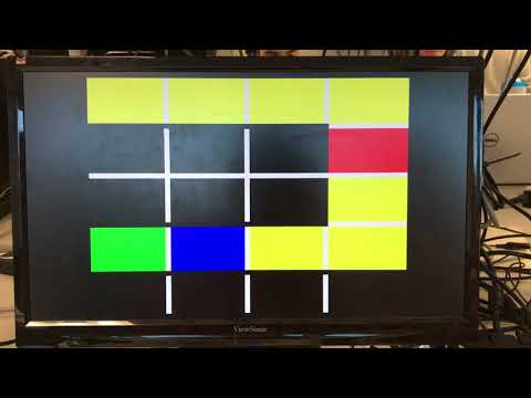
The last part of updating the display was receiving the done signal. Once we got this signal from the SPI we changed all unexplorable locations to black to display the robot has completed its maze exploration stage. To do this we simply checking all the locations that were still untraveled and changed them to untraveled. We could do this because if they were travelable then our robot would have visited them already.

Audio

When the robot is done exploring the maze, it sends a done signal to the base station. Along with updating the untravelable locations as mentioned before, this also triggers a 3 toned tune to play signaling the maze exploration is complete. To make this tune we converted our code from lab 3 into a Tune module and added that to our project. This code plays a 200 kHz sine wave tune for one second, then switches to a 400 kHz sine wave tune for a second, and finally plays a 700 kHz sine wave tune for a second before repeating itself. In order to play these tunes, we created a table of 629 sine values and iterated through them at the specified frequencies to get the tones we wanted. We struggled to get this working and we figured out we had to manually connect our pins from DE0_NANO straight to the SINE_ROM we created instead of trying to connect it through the Tune module. It worked perfectly after we did that, though, as illustrated by the video of the full setup above.

Building the robot:

Team members:

Logan, Yonghun, Francis

Materials Used:

Arduino
Calvin
PCB Mill and Copper
Laser Printer

Line Sensors: As stated in milestone 3, we decided to implement a new line sensor, the Pololu QTR-8A Reflectance Sensor Array, to our robot. In order to be able to use all 8 of the line sensors, we had to add a mux to it. We soldered the pins of the line sensor to the corresponding pins of the mux.

We started off by testing each of the 8 line sensors using the serial monitor. We printed the analogRead of each of the line sensors to see their values for black versus white. In order to read all the values, we created a function that set the select lines s0, s1, and s2 to the corresponding values for each line sensors.

However, we ran into problems with the output values from the mux. We realized that we were not getting the correct readings from the mux that we were getting if we read directly from the line sensor. We realized our mux was probably broken which created a huge problem since it was soldered onto our line sensor. The lessons we learned from this experience was
1) do not solder the mux directly onto the line sensor and
2) order a back up line sensor just in case something goes wrong with the first one.

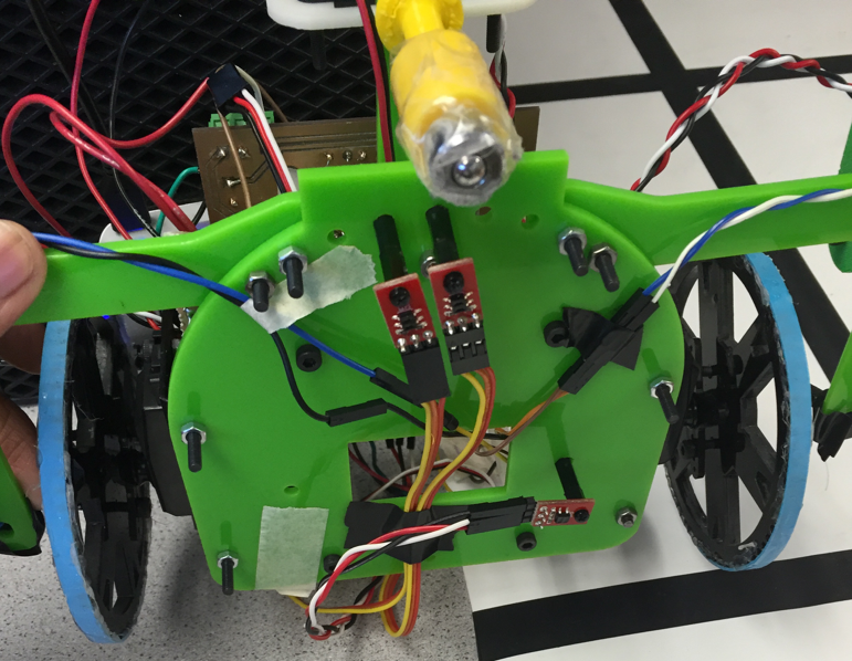
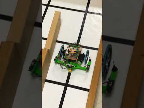
Since we could no longer use the Pololu QTR-8A Reflectance Sensor Array, we decided to attach three of the line sensors provided in lab to the bottom of our chassis as seen in the image below. The two line sensors in the front are for line following and the line sensor to the side is for intersections.

In addition, we decided to use a Schmitt trigger for the wall sensors so that we could use digital pins for those inputs, thereby freeing up analog pins for other purposes.

What is a Schmitt trigger and how does it work?
A Schmitt trigger is essentially an opamp with positive feedback. Normally we connect an opamp with negative feedback because otherwise its extremely high gain would cause its output to uncontrollably go up to the positive rail (Vdd) or fall down to ground. In a schmitt trigger, though, we use the two resistors as a divider to set the voltage at which this occurs. If the input voltage is higher than a certain value, the output immediately spikes up to Vdd and if it is lower than a certain threshold, the output drops. This behavior can be very useful in converting an analog voltage to a digital one which only accepts HIGH or LOW. For our Schmitt triggers, we chose to use the SN74HC14.

It is an inverting Schmitt trigger; on the datasheet it explains how the analog input values will correspond to the output.

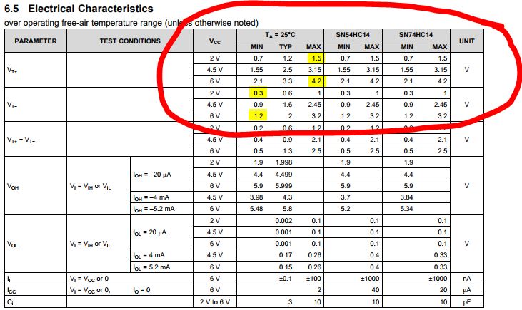
The highlighted values are very important in understanding how the trigger will operate. Vt+ is the threshold voltage to be recognized as a logic high input: any voltage higher will be considered logic HIGH. Similarly, and voltage below Vt- will be recognized as logic LOW. We can see from these specs that if Vcc is decreased, the threshold voltages decrease.

When probing the output of the wall sensor, we found that it rose to ~2V when the wall was present and below 1V when there was no wall. This output of 2V for high would not be high enough to be recognized as logic high by the schmitt trigger if it was powered from 5V, but may work correctly if it was powered from 3v3. After testing with the Schmitt trigger, we found that the wall sensor readings worked perfectly if the Schmitt Trigger was powered from 3v3, but not at all if it was powered with 5V, as predicted by the datasheet.

Treasure and Wall Sensors Placement:

In order to place our treasure sensors in the optimal location, we laser printed “wings” to robot to mount our two side wall sensors and two treasure sensors. Since we want the treasure sensor to be around 4cm off from the ground and in line with our intersection line sensor, we printed wings to place our treasure sensors exactly there.

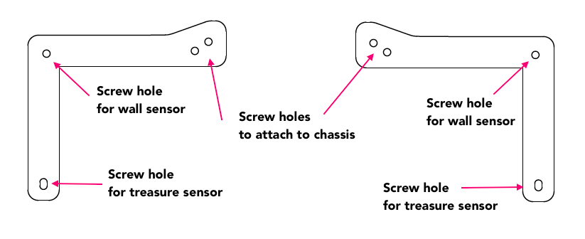
In order to facilitate the revamped design with the Schmitt trigger, no muxes, and a different number of sensors, we decided to redo the PCB design. The plan was to create an Arduino Shield which would have screw terminals for all of the sensors, a socket for the Schmitt Trigger IC (SN74HC14), two pushbuttons, and two LEDs. The main goal was to minimize the wiring headaches we had been struggling with for the past few weeks, to set the wiring now and never change it again. We recommend using the following image from this website to measure out the hole spacing.

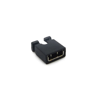
As with any PCB, it began with a schematic. While a full PCB tutorial is beyond the scope of this site, there are many good options online. We prioritized modularity in the design so many pins were connected through two-pin headers, allowing us to connect and disconnect the pushbuttons, battery, and LEDs at will using the small header short pictured below. This offers the robustness of a PCB, while still being modular like a breadboard. We highly recommend using these for simple PCB designs:

The schematic of our new PCB is shown below:

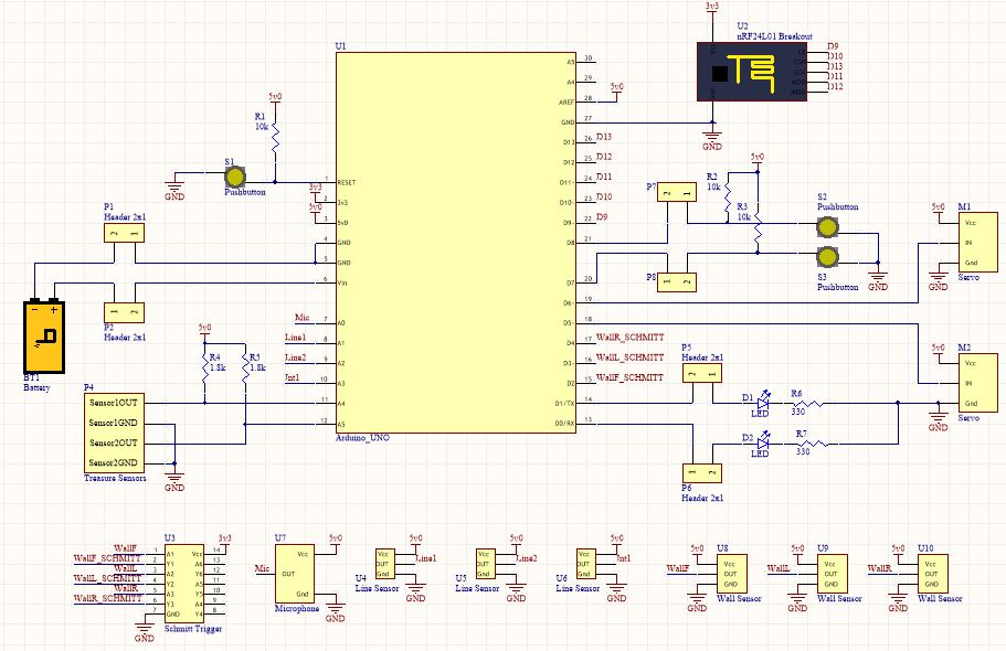
*Note that the pins on the Arduino in the schematic do not correspond to actual pin numbers but rather pad locations for the layout

The PCB design is shown below:

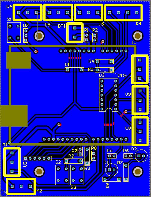
Manufacturability and space were the two primary concerns because we decided to mill the board in the Maker Lab so we needed to be wary of its tolerances and its cost. The copper is expensive so we wanted the board to be as small as possible while still accommodating all of the necessary components.

*Note the Arduino is shown as if it were on the bottom layer because it will be flipped over and plugged into the board

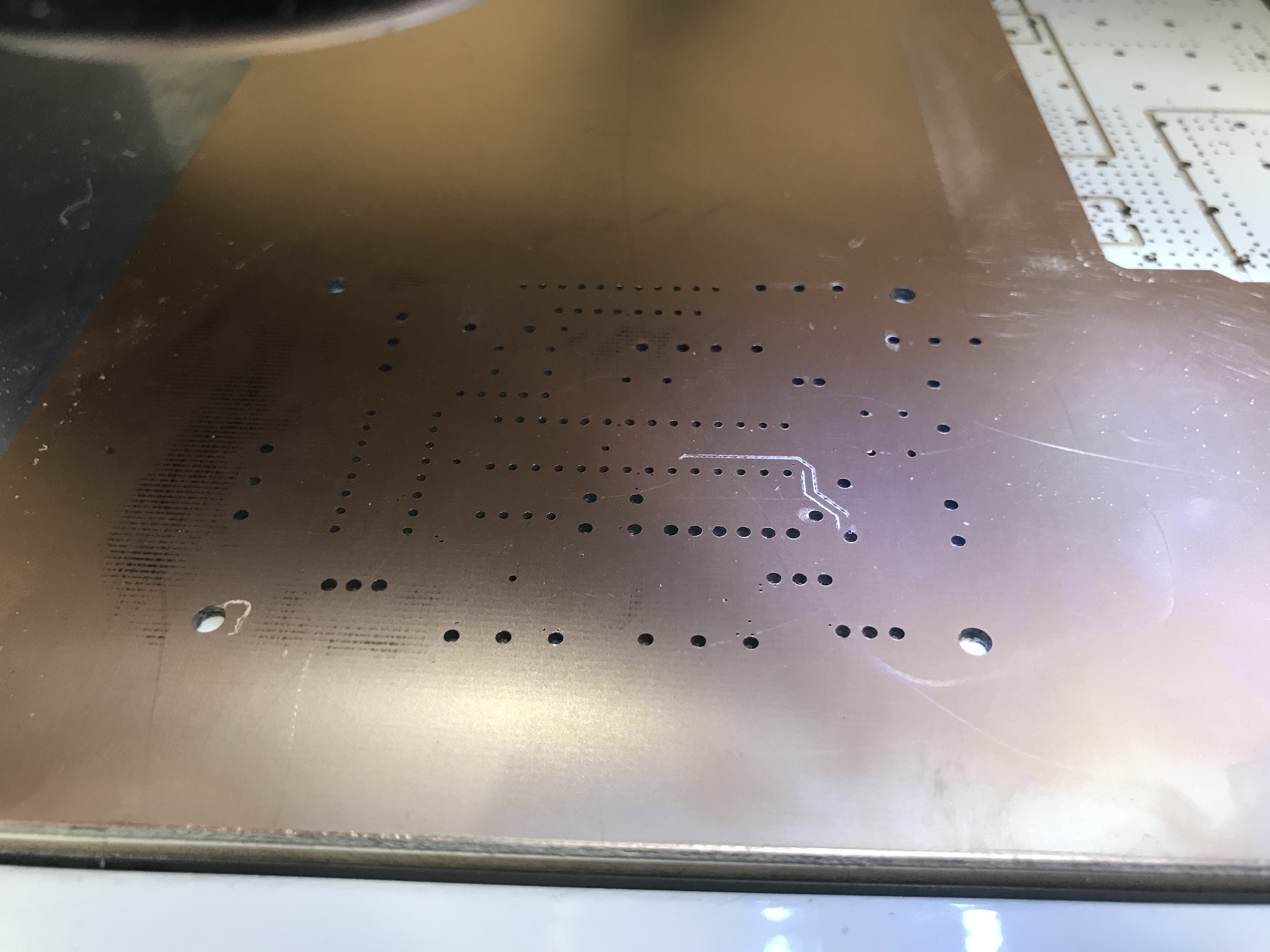
Next, we needed to mill the board. This consists of cutting away the copper between traces and around drill holes so that various parts of the boards are not shorted together. First, we run the drill layer and end up with the following result:

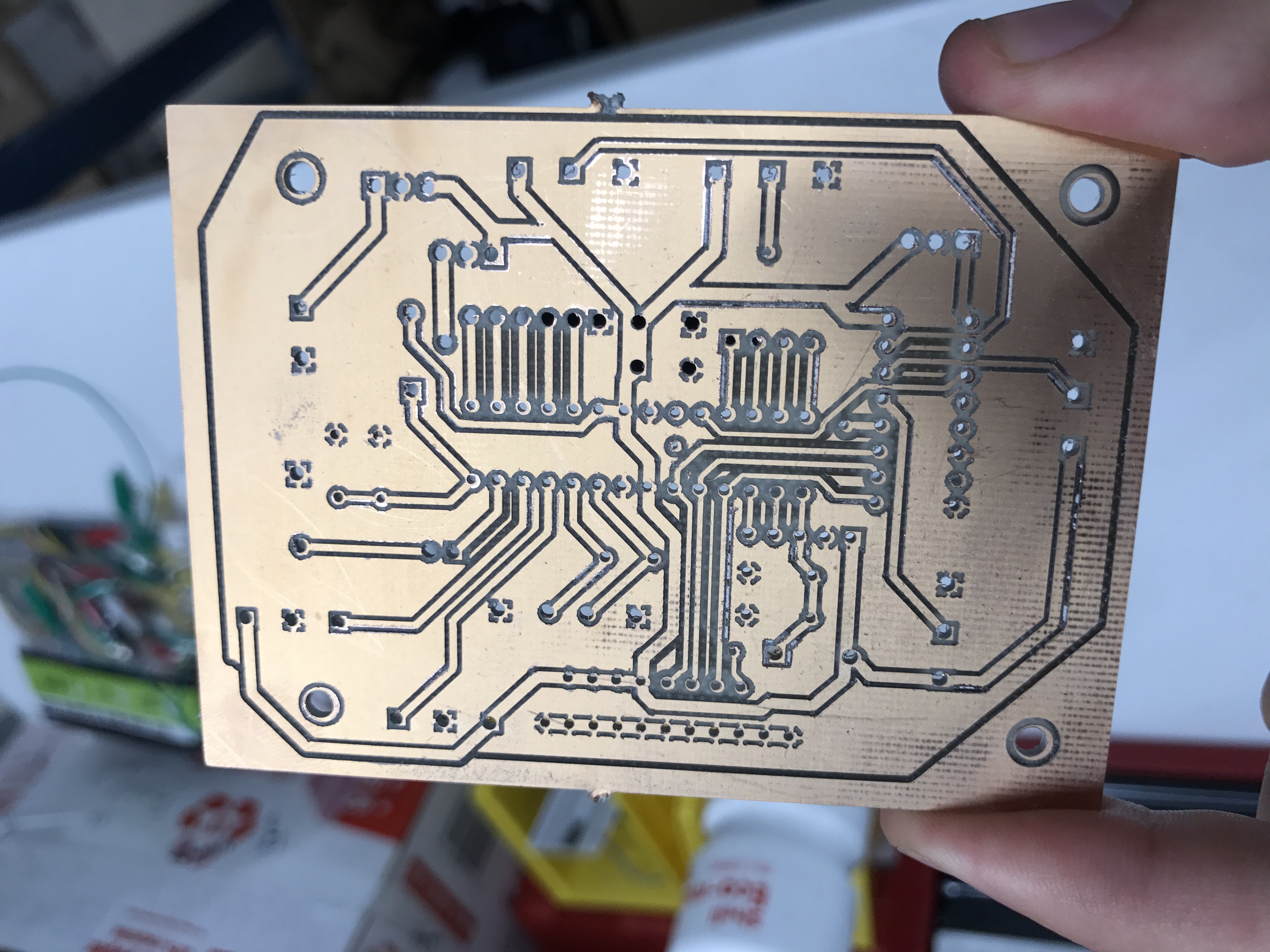
Then we run the top and bottom layers which cut away copper until we have traces between the drill holes and leaving something which lookes like the following image. The black lines are places where the copper has been cut away, creating thin copper traces between.

Next, we need to populate the board. This consists of gathering all the components and soldering them on, verifying their location using the schematic and layout pictured earlier.

After soldering them on, it is extremely important to test the connections. Using a multimeter you should:

Visually inspect all solder and check that nothing crosses over isolations
Check continuity between the component and the trace it is soldered to (Should be <1ohm)
Check continuity between the trace and adjacent ones (Should be infinite resistance)
If the bottom is a ground plane (which it was in our case) then check the resistance between the soldered component and ground (Should be infinite unless they are connected via resistor)

*Note: When turned off, a voltage regulator will actually create a non-infinite resistance between ground and the 5V trace. (about 13k in our case)

After verifying all of the traces in the above process, you are still not ready to attach electronics. Now you should do the initial power-on test. Wire up a battery or DC voltage source to the input terminals on the board and verify that all power rails are at the proper voltage and the input current is reasonable for what is connected.

Finally, you can attach all of the electronics and continue the testing procedure. In our case, this consisted of checking the input and output of every pin on the Arduino, ensuring that it was connected to everything properly. The first test we did was run Blink() with attached LEDs:

We were successfully able to incorporate the PCB onto our robot for this Milestone, but found that there were issues with Calvin’s movement even though we verified the motor connections. We realized that our single battery could not power the motors, Arduino, and all the sensors. We decided to add a second battery just to power the motors. Of course the PCB was already designed and manufactured, so we needed to add a small perfboard to hold the screw terminals and voltage regulator.

Outcome

We completed this Milestone in two parts:

Finalize the communication protocol and display everything to the screen
Map the maze with Calvin

Part 1 was completed flawlessly as depicted in the videos above.
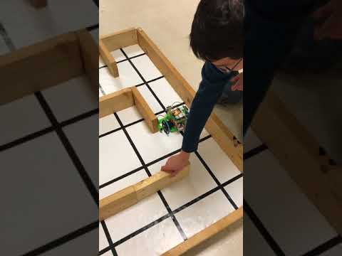
Part 2 was hindered by our inability to get the algorithm fully functional. Also, the treasure sensors were unable to detect treasure while it moved throughout the maze, though detection at a standstill worked fine. We were able to explore the maze with a simple algorithm using wall detection and simply choosing to go straight unless blocked, in which case Calvin would go left unless blocked, then choosing right and finally backwards. Here are a couple runs of that:

TODO:

Our next step is to fully incorporate our modified DFS algotihm so that Calvin can correctly map the maze and signal when he has done so.
We need to implement the mobile treasure sensing.
Finally, we need to check the full communication pipeline over radio while Calvin is mapping the maze.