Lab 9 Mapping
In this lab we build a map of the wall and obstacle lab space set-up by placing the robot at five different locations and measuring the ToF sensor readings while spinning the robot about its axis. We used transformation matrices to merge all the readings and plot the final map. The map created in this lab will be used in future labs involving localization and navigation tasks.
Orientation Control
The first step was to allow the robot to turn on its axis in order to get the maximum number of ToF sensor readings. I chose to do PID control over the orientation instead of the angular speed control. I executed Task 2 for Labs 6-8 and had a working PID controller for rotating the robot. After making minor changes to limit oscillations and jerks, I was able to use the same PID controller code to make on-axis turns in small increments. First, I programmed the robot to turn 20 degrees and eventually 10 degrees. To take a full 360 degrees turn, the robot repeats the rotation action 36 times, running a PID loop for each 10 degrees rotation. This process required a lot of trial and error to tune the PID controller as the battery voltage really affects the speed ranges and coefficients. I also ensured that the robot does not drift too much from its starting position while executing the on-axis turn, where one set of wheels moves forward and another set of wheels moves in reverse. I have not included a set point graph as the same PID controller from the previous labs is used. From the yaw angles calculated using the gyroscope values, the change in yaw in each rotation is slightly less than 10 degrees. However, while completing a full 360 degree rotation the robot returns back to its original position. This might be because of inaccurate gyroscope readings and drift due to one set of wheels moving faster than the other (tuning in lab 5). As we are moving the robot in a large number of increments and the rotation angle is small, I chose to ignore this minor discrepancy and assumed that the robot moves uniformly in angular space. The video below shows the robot rotating on its axis in 10 and 20 degree increments.
To perform the ToF sensor measurements, the robot first takes the ToF sensor reading and then rotates. There is a small delay after the rotation movement to ensure that the robot is still before taking the next measurement and repeating the same. The robot repeatedly polls the sensor to get three readings and stores the average. Note that the ToF sensor runs in Long Distance Ranging Mode as it is the most suitable for the size of the lab space setup. Given that my ToF sensor is not very accurate (lab 3), using the orientation control method is better as the sensor reading is taken when the robot is still and guaranteed to be pointing towards a fixed point in space.
The drift in the gyroscope sensor readings did not affect the PID controller because the PID controller is restarted for every single 10 degree rotation. When the PID controller is restarted the yaw angle calculated is taken as the 0 degree (initial angle) and the PID controller rotates the robot by 10 degrees. As this rotation takes very little time, the drift does not affect the yaw angles. If I had chosen to keep the PID controller running, then the sensor drift would have had a significant effect. While the robot does return to its original position in a full 360 degree rotation, it does drift a bit towards right while rotating on the floor . Considering the size of the robot (18 cm) and drift during the on-axis rotation movement, we can say that the ToF can deviate a maximum of 10 cm from its intended circumference of on-axis rotation. So the map would have a maximum error of +/- 10 cm.
Read Out Distances
We had to execute the turn at all five of the marked positions in the lab space setup. Given below is a plot of the lab space setup and the marked positions. I used the code in the provided lab 10 simulation package to generate the lab space setup. As the positions in the lab space set up used a 1 ft x 1 ft grid scale, I have used ft as the unit for all my readings and calculation.
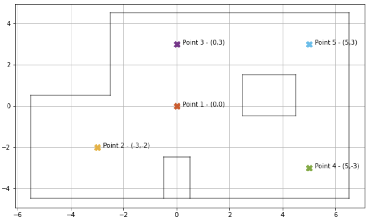
I placed the robot in the same orientation at each position, the front ToF sensor facing the left side (180 degree angle). As the PID controller rotates the robot in clockwise direction, the readings are taken from 180 degree to -180 degree in degree increments. While completing the turn at each position, the robot stores the distance and orientation at each increment. On sending the “GET_DATA” command this data is sent over via Bluetooth. Initially I had set the robot to send the data over as soon as the turn was completed, however I faced a lot of issues with Bluetooth getting disconnected while performing the turn. To avoid losing data in such a manner, I added the “GET_DATA” command. As mentioned in the previous section, based on the robot’s behavior, it is reliable to assume that the readings are spaced equally in angular space.
In order to check that the robot scans are precise, I rotated the robot twice and four times at (0,0) point. Given below are the ToF scans for two rotations and four rotations. I noticed that the sensor readings were very noisy and not consistent
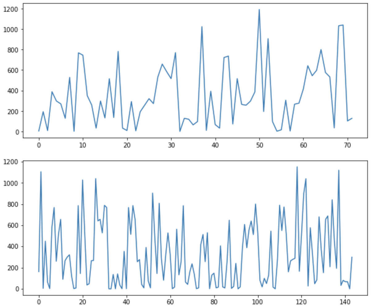
Owing to lack of time and inaccuracies with my ToF sensor at this stage, I collaborated with two other classmates (Krithik Ranjan and Aparajito Saha) in order to collect data. They had used a similar strategy to perform the turn. While we used a common robot to get the readings, the plots and analysis were all done individually.
For every point, I generated a simple plot of the ToF sensor scans against time as well as a polar plot for the ToF scan and the orientation angle it was taken at using the matplotlib package. Note that I had to add a sensor offset to the readings to account for the sensor being placed at the front of the robot (72 mm away from the center) and not at the center.
-
Point 1 - (0,0)
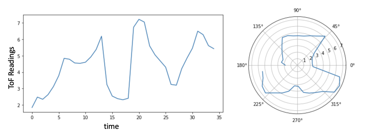
Fig 3: (1) ToF Sensor Scan (2) Polar Plot -
Point 2 - (-3,-2)
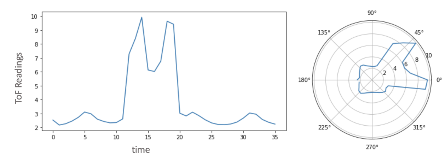
Fig 4: (1) ToF Sensor Scan (2) Polar Plot -
Point 3 - (0,3)
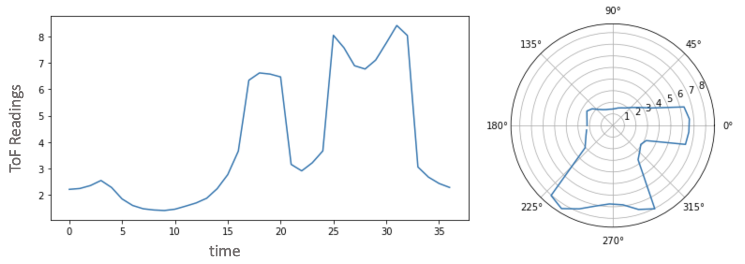
Fig 5: (1) ToF Sensor Scan (2) Polar Plot -
Point 4 - (5,-3)
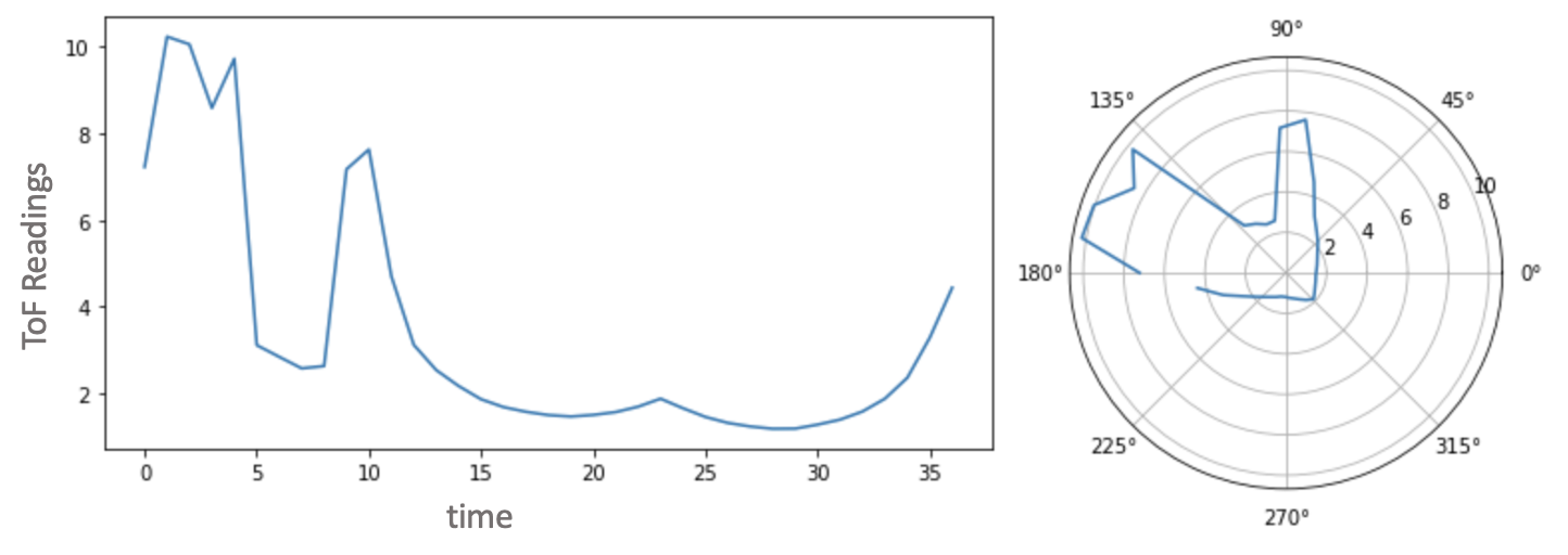
Fig 6: (1) ToF Sensor Scan (2) Polar Plot -
Point 5 - (5,3)
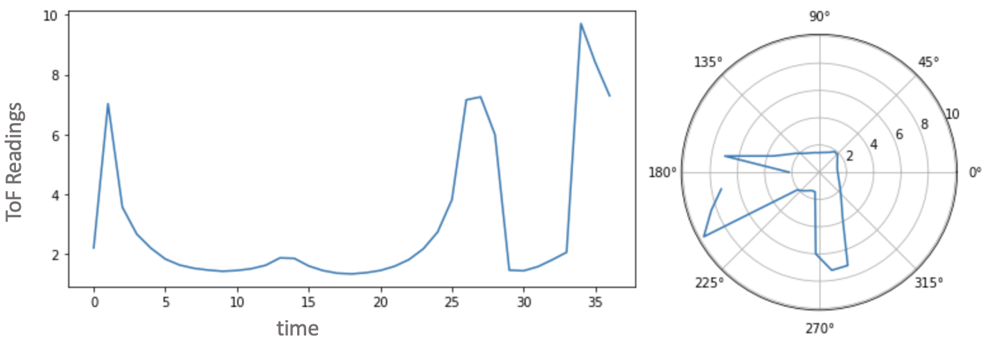
Fig 7: (1) ToF Sensor Scan (2) Polar Plot
Merge and Plot
The final and the most important step of this lab was to convert the measurements from the distance sensor to the inertial reference frame of the room. The lab space is to be mapped as a 2D grid using cartesian coordinates. The ToF sensor readings combined with the orientation/angle of the robot can be interpreted as polar coordinates. First, I converted the readings to cartesian coordinates as (r * cos(a), r * sin(a)), where r is the sensor reading and a is the orientation angle. As each of these cartesian coordinates were taken from different points in the space instead of just the origin, we need to use translation transformation matrix to convert the measurements to the inertial reference frame of the room. In the transformation matrix, Tx and Ty are the coordinates of the position from which the turn was executed.
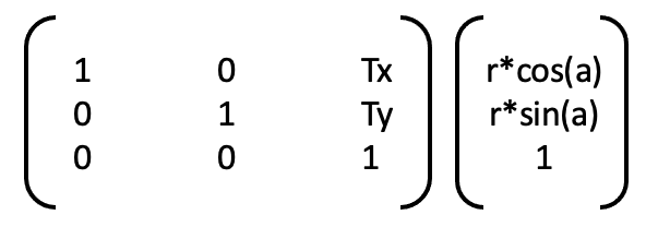
For each position, I transformed the readings and then created a scatter plot using matplotlib. Given below are the scatter plot for the readings from all five of the positions, I had used different colors for reading from different positions; and added the true plot of the lab spacing for reference.
-
Point 1 - (0,0)
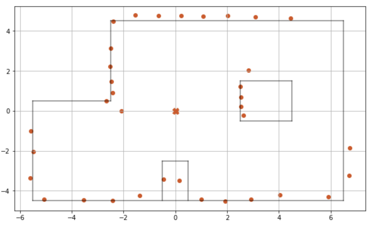
Fig 9: Scatter Plot -
Point 2 - (-3,-2)
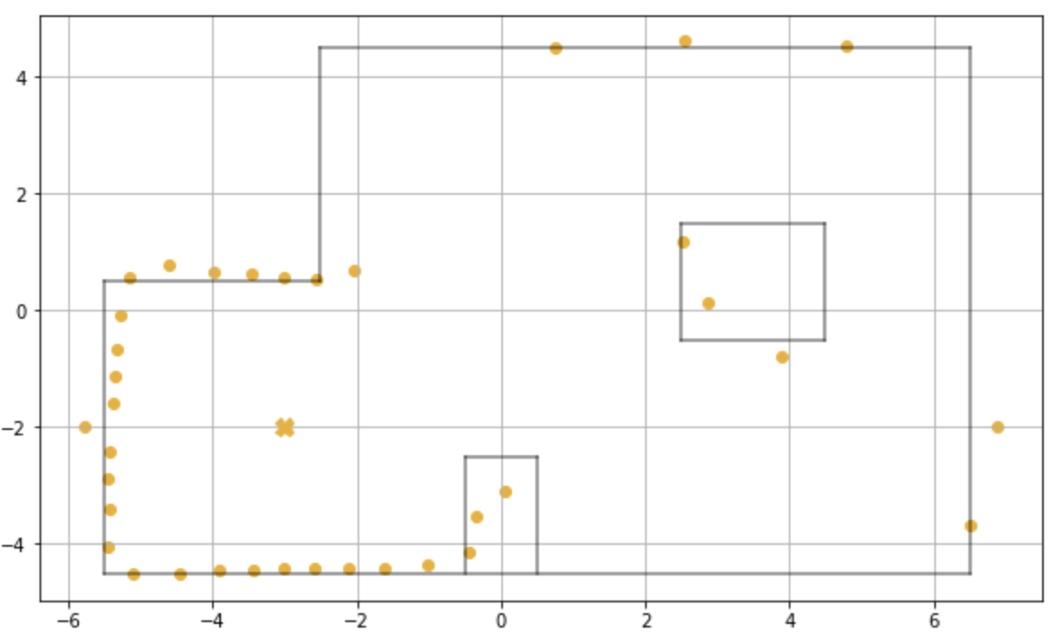
Fig 10: Scatter Plot -
Point 3 - (0,3)
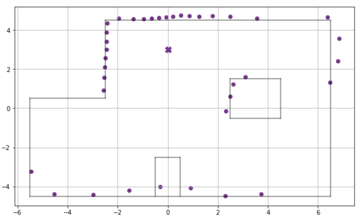
Fig 11: Scatter Plot -
Point 4 - (5,-3)
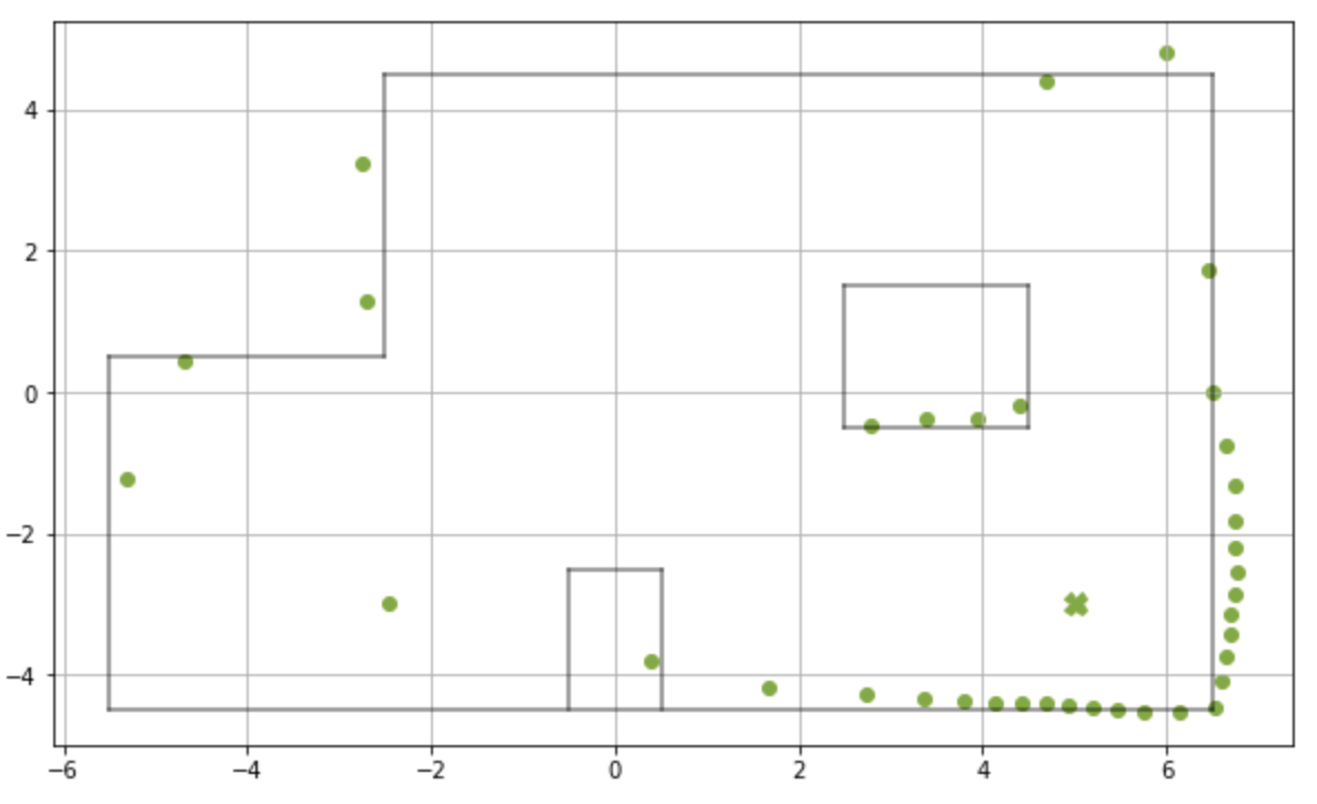
Fig 12: Scatter Plot -
Point 5 - (5,3)
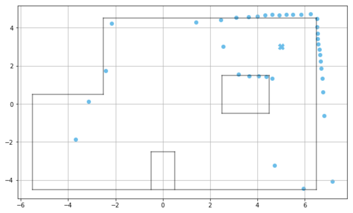
Fig 13: Scatter Plot
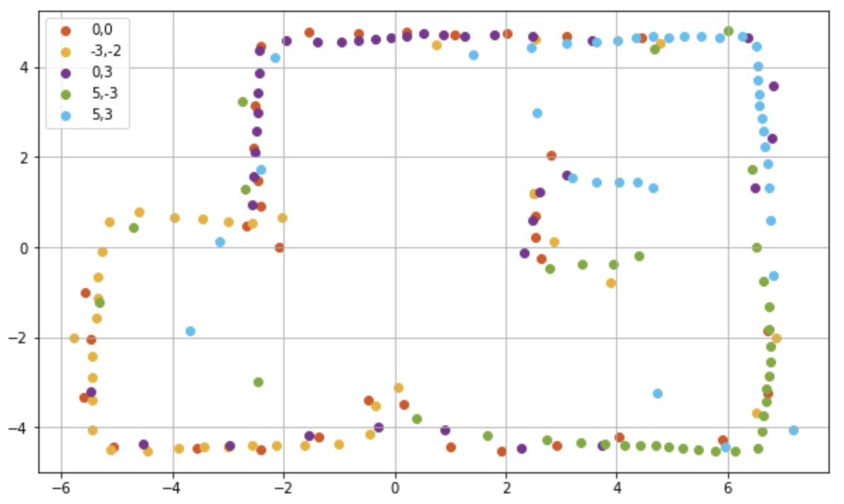
Below is the combined scatter plot of all the readings. While there are plenty of data points for the walls of the setup, there were very few data points for the top edge of the small box kept at the bottom and the right edge of the box in the middle. The right edge of the box in the center is a blind spot for the sensor as it can only be seen from positions (5,3) and (5,-3) where it only measures the top right and bottom right corners of the box. However the bottom box is covered from four positions and should have enough data points in theory. As the box is very narrow, from far away point (0,3) it is within 10 degree angular space, so only one data point will be measured in its region. From the origin, (-3,-2) and (5,-3), there are about three data points each for the box but are inconsistent and do not provide an accurate representation of its positions. The material used for the wall/edges was wood, whereas cardboard boxes were used for the obstacles. As the sensor behaves differently for different materials, the discrepancies in sensor readings are higher for the obstacle boxes.
Converting to a Line Based Map
To convert the scatter plot to a line map, I first grouped the data points that formed each edge. I sorted the points according to the x coordinate to group data points the vertical edges and then by y coordinates for the horizontal edges. I did remove some of the out of the way datapoints. I used numpy’s polyfit() and poly1d() function for linear regression to find the best fitting curve for the set of data points for each edge. The plot below displays the linear regression lines in red.
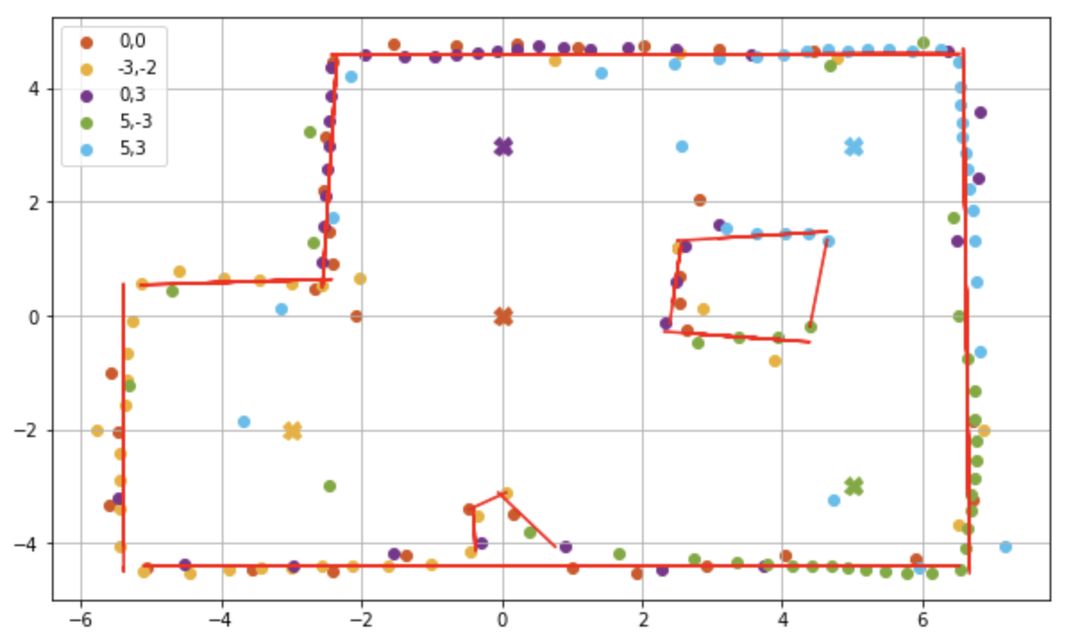
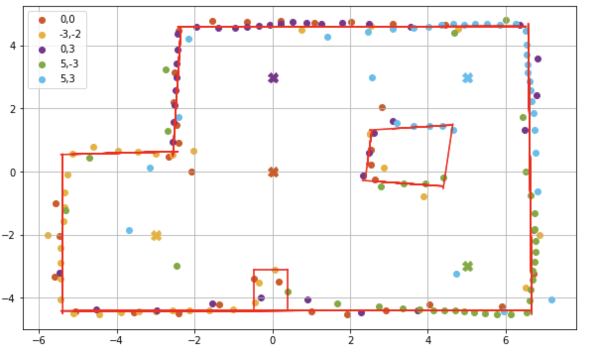
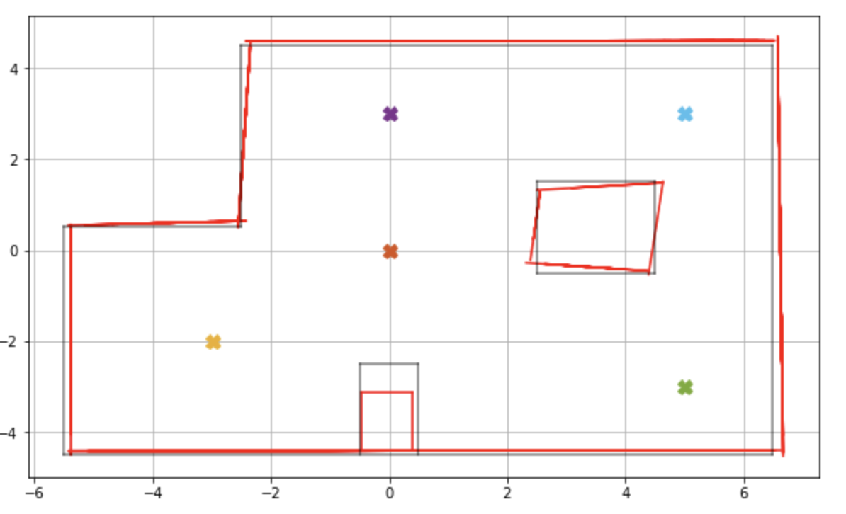
I extrapolated each of the individual edge lines and joined them to form the graph below. I made some adjustments to the bottom box edges. As we know that the obstacle is made of 90 degrees, I used the left most, right most and top most data point in the box area to form the edges for the obstacle. The final mapping is in red and the set up map is in black.
Conclusion
Comparing the mapping with the actual map of the lab space, we see that the mapping has the general layout of the lab space, barring the bottom obstacle. The final lines are a little shifted towards the right, this could be due to the right drift of the robot mentioned earlier. I have saved the line endpoints to be imported in the simulation. I am happy with the results of this lab and I hope this mapping will suffice for the future labs.