In this lab we were introduced to the simulation environment and learnt how to programatically control a virtual robot and analyze its movements uusing the live plotting tool. We will use this simulator in upcomming labs to test the localization algorithms before implementing them on the actual robot.

Simulation Environment

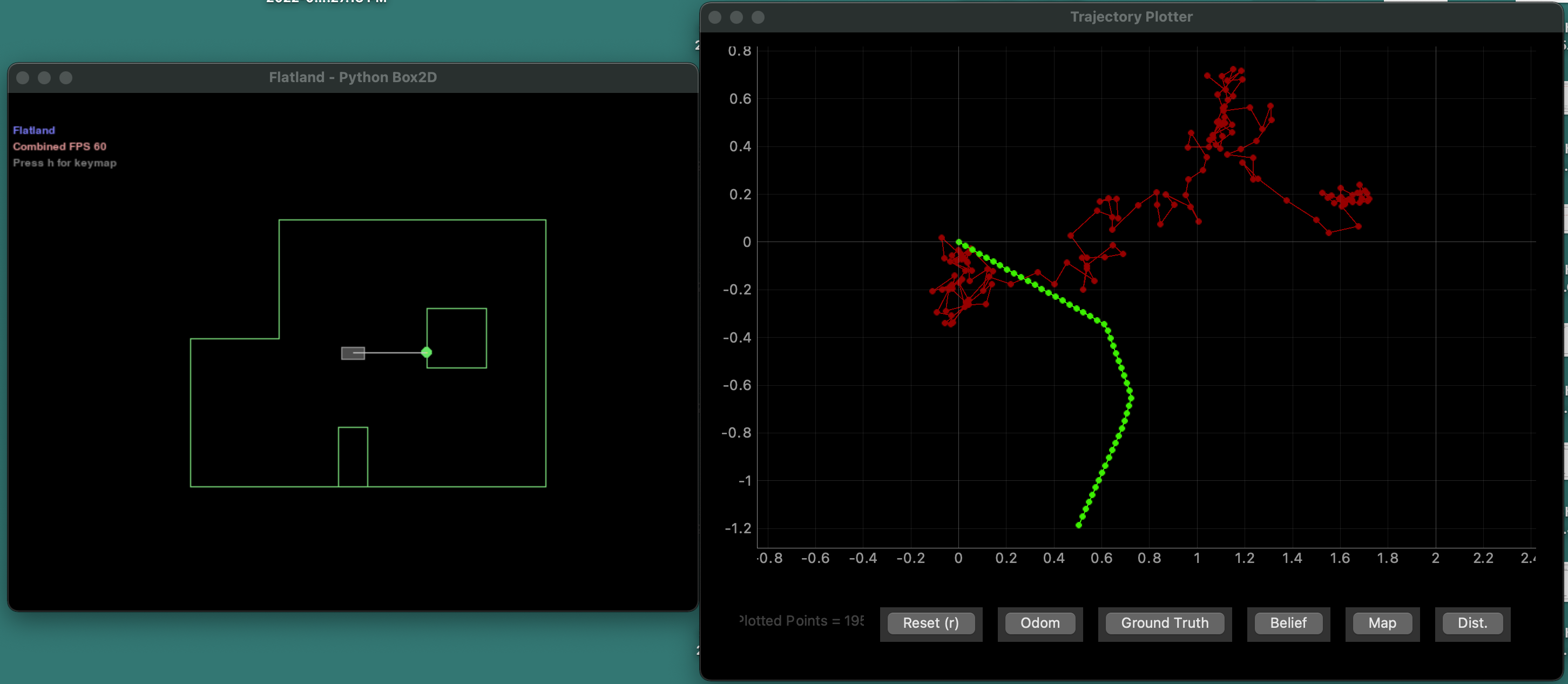
To setup the simulation environment, I had to upgrade my python version, install few packages and download the simulator base code and lab 10 notebooks provided. The Simulation Environment consists of three components - (1) Simulator, which simulates the virtual robot equipped with laser range finder that moves in the virtual world similar to the lab setup, (2) Plotter, a 2d plotting tool for live asynchronous plotting of the odometry and ground truth poses of the robot, (3) Controler to control the virtual robot using the provided Python API interface. We can used the commands in the Commander class to access data or plot in the simulator. We can start the simulator and plotter (shown in the image below) programatically or using the GUI buttons. I played around with it by driving the robot using keys (up and down keys to change the linear speed and right & left keys for the angular speed). I noticed how the ground truth plotted on the plotter in green follows the actual movement of the robot, but the odometery plotted in red, which is the perception of the robot's position based on its sensor values is very inaccurate.

Open Loop Control

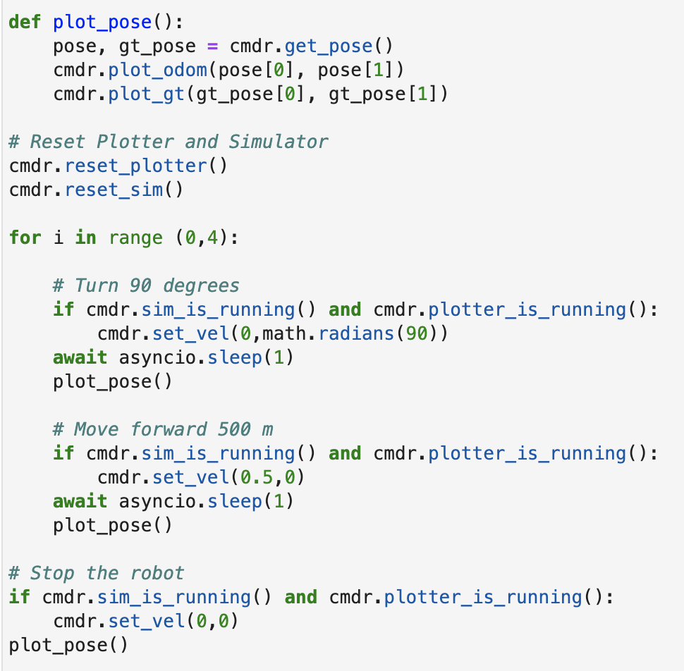
For our first task we had to program the virtual robot to execute a "square" loop. I first played around with the cmdr.set_vel function to gauge the duration of the velocity command. This function takes in two variables, one for linear velocity which moves the robot forward or backward and one for angular velocity which rotates the robot. The unit for linear velocity is in meters per second and the unit for angular velocity is radians per second. This means if use cmdr.set_vel(0.1,0), the robot will move forward at a speed of 1 cm in 1 second. To execute the loop, I gave the following pair of command four time to create the four sides of the square - [Turn 90 degrees, Move forward 50 cm]. For the robot to turn 90 degrees, we have to set the angular velocity as 1.57 radians/second and wait for 1 second. Similarly to move forward, we set the linear velocity to 0.5m/s and wait for 1 second. Note that I had to ensure that the plotter and simulator were still running before each step. I also created a function called plot_pose to plot the ground truth, this was also called after every command.

The video below shows the robot executing the action.

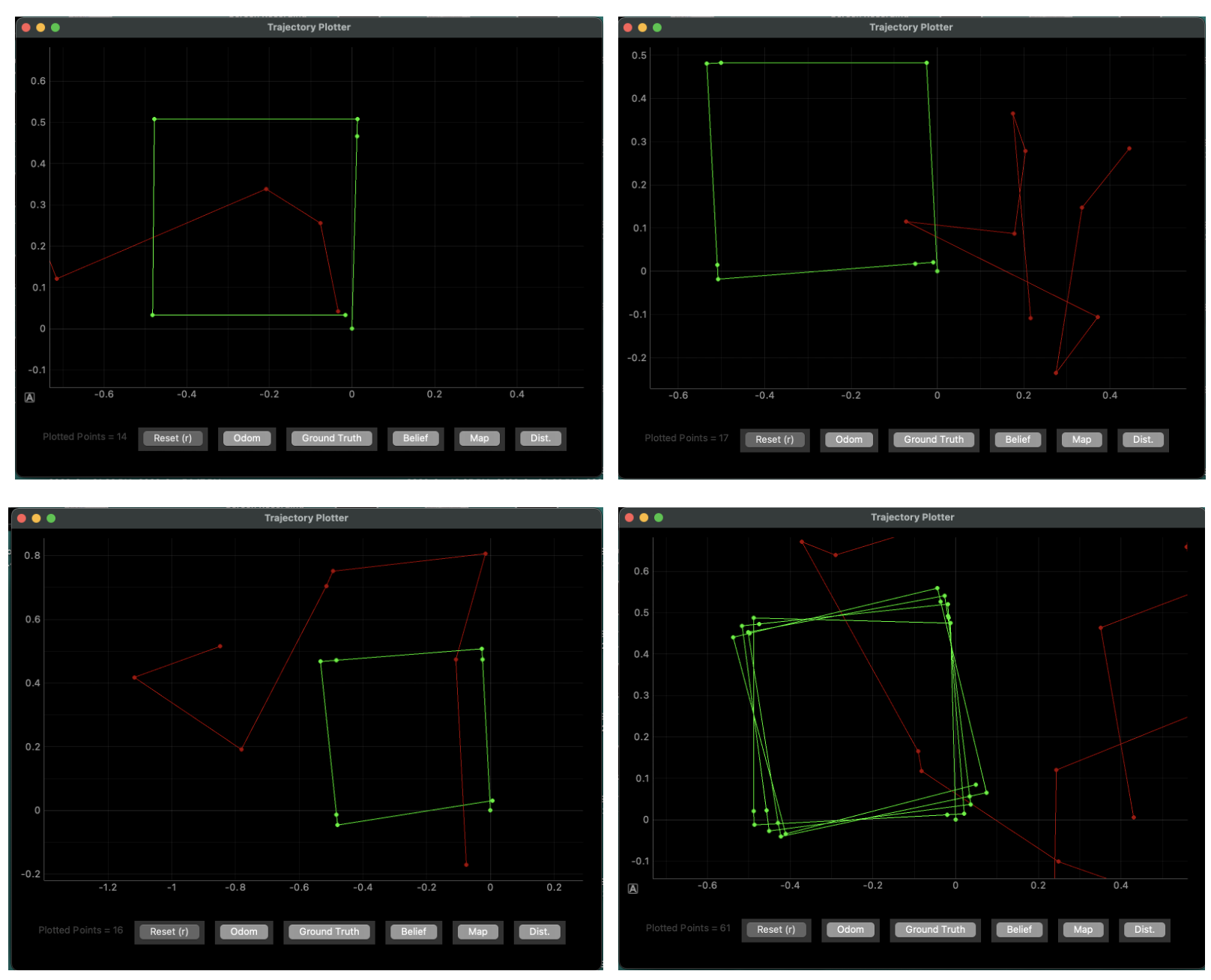
The first three images plots of the robot executing the same task three different times. Note that the "square" created is different every single time, the angles might not be exactly 90 degrees and the distance travelled might not be exactly 500 cm. This is because we are using await asyncio.sleep(1) for the time delay, which is not accurate and can result in different waiting times. So the velocity is command is never run for exactly 1 second, so angle turned and distance moved is never exactly 90 degrees and 50 cm. The last image is a plot of the robot executing the square four times. As exepected the shapes are distorted in this plot as well.

Closed Loop Control

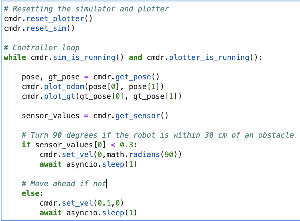
For our next task, we had to design a simple controller to perform a closed loop obstacle avoidance task. We will used the sensor reading from the front ToF sensor to detect obstacles. To start, I created a simple controller, which checks the current sensor reading. If the robot is less than 30 cm from an obstacle, it stops moving forward and turns 90 degrees. Otherwise, the robot moves straight forward with a speed of 10 cm per second for 1 second. I chose 30 cm as the obstacle distance because it gave enough room for our 20cm long robot to make a complete uturn (accounting for the drift). In the video below we can show the robot executing this controller. The robot can get as close as 30 cm without colliding with an obstacle.

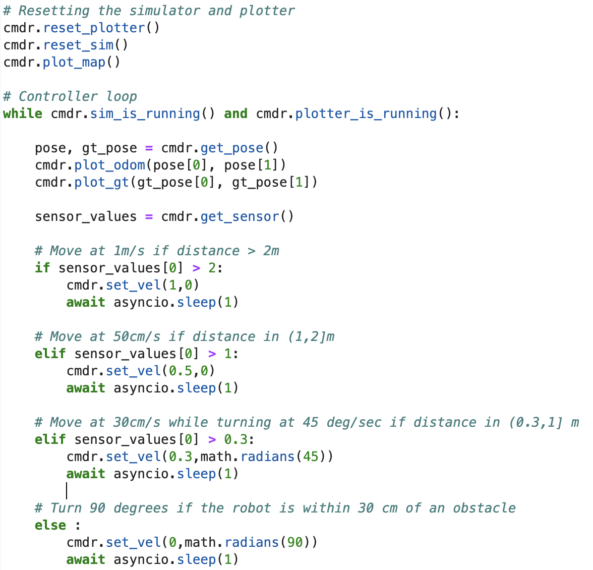
While the above controller pefectly avoids obstacles, I feel like it is too safe and moves too slowly. I improved this by changing the linear speed of the robot based on how close it is to an obstacle. If the obstacle is more than 2m away, the robot moves with a speed of 1m/s. If it is within 2m - 1m, it moves with a speed of 0.5m/s. If it is within 1m - 30cm, it moves with a linear speed of 30 cm/s and rotates with a speed of 45 degrees per second. This combined translation and rotation motion, helps the robot avoid an obstacle before it is too close to it, as the robot is already searching for a new location by rotating. However if it reaches within 30 cm of an obstacle it makes a sharp 90 turn. This controller is much faster and minimizes collisions due to the rotation technique described above when it is in nearing an obstacle.

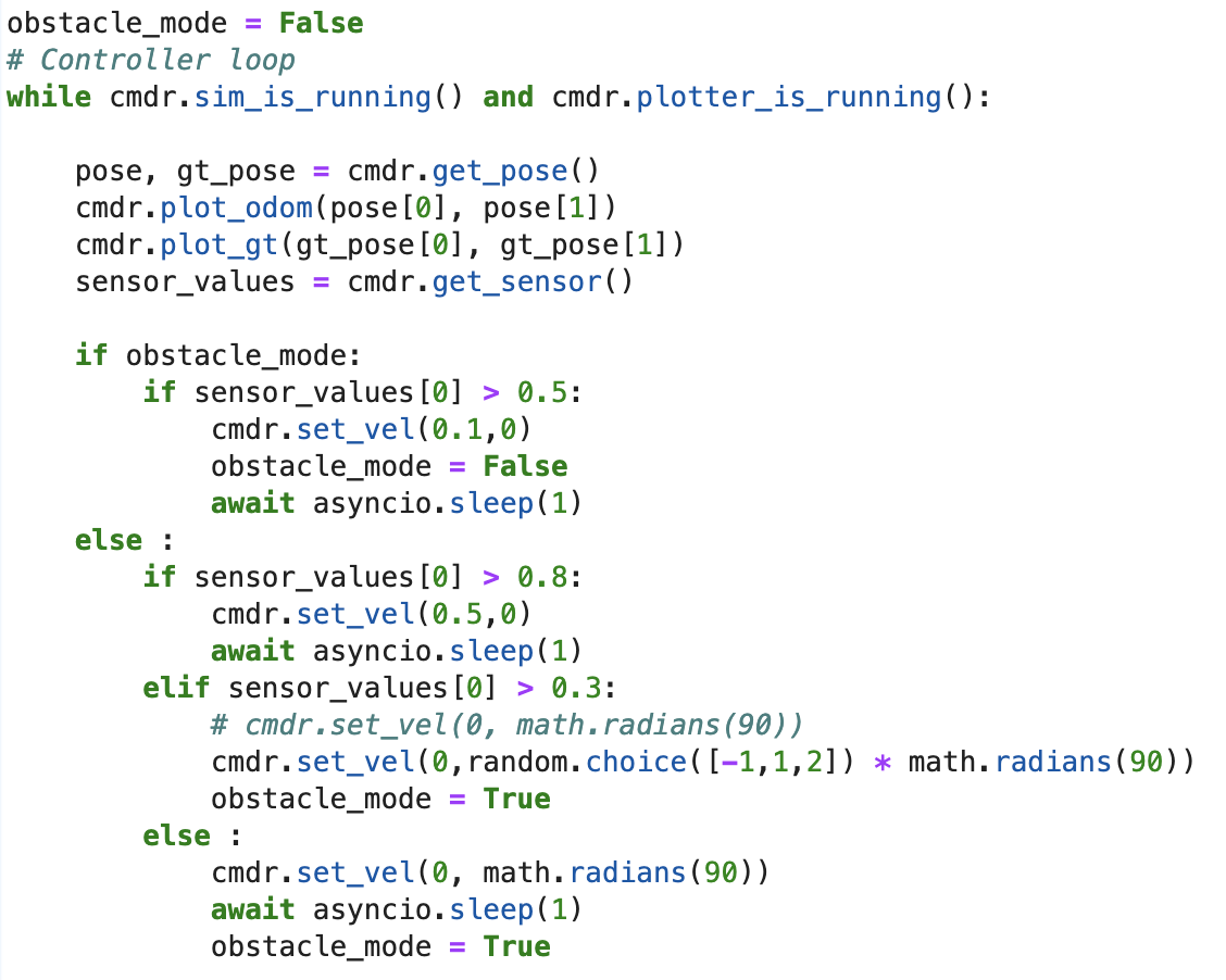
However in the controllers described above, they ignore the fact that the robot's sides could collide with the obstacle. For example, if the robot is on the left side of the bottom obstacle at a 45 degree angle, it sensor value will be large as it points towards the top edge of the maze. However if the robot moves forward, its right side will collide with the obstacle. To avoid this, we would need to do a sweep of the location to ensure that no part of the robot can bump into any obstacle. I implemented a simplified version of this controller. If the robot is close to an obstacle, it is in obstacle mode. It starts to turn at a speed of 90 degrees per second. There is no wait period, the robot keeps checking if has 50 cm away from an obstacle. If so, it gets out of obstacle mode and moves 10 cm with a speed of 10 cm/s. I found that this controller worked the best and avoided the most of the obstacles. To add some randomness into the movements, I also added a random selector for the angular speed (90 deg/s, 180 deg/s and -90 deg/s).

Thanks to the Prof Petersen for allowing us to work on this lab during lecture and to Vivek for creating and explaining the simulator to us.