library(tidyverse)
library(skimr)
library(tidyverse)
library(tidymodels)
library(openintro)New York Traffic Accidents
Report
Introduction
We picked the US-Accidents: A Countrywide Traffic Accident Dataset for our project because we believe that understanding what factors are associated with higher severity of accidents and what may make an accident have a larger delay on traffic could provide critical insights that can be used to make our streets safer, and for transportation and gps companies to be able to more effectively plan the best routes for their customers. Due to its uniquely dense arrangement and construction layout, New York state has seen an unparalleled level of traffic accidents, despite its effective urban planning. Our project focuses on understanding the factors contributing to this trend --- we picked New York Traffic Accidents as the topic given that we believe that analyzing which factors are associated with higher severity of accidents and that cause significant travel delays could provide critical insights to make our streets safer. Moreover, transportation systems and navigation applications would also effectively analyze and map-out the most efficient and reliable routes for their customers, transforming the way we travel through one of the most bustling cities in the world.
This dataset contains important variables such as severity of accident, weather/precipitation and time of day which can help us answer our research question of “how does the weather (specifically weather condition) and time of day when accidents occur in New York state affect the severity of the accident”. The context of our work is traffic accidents in New York state based on weather and time of day. By our results from the models and hypothesis testing, we can see that our results have conflicting results. We can begin to see that our hypothesis that bad weather or time of day increases the severity of an accident is possibly correct by our hypothesis tests. But, our logistic regression exemplifies that this is not the case.
If we were given 6 months and \$500,000 to work on this project, we would continue to find out why our results are conflicting. In the future, we would love to explore the relationship between such variables in different parts of the world where their infrastructure and layout is quite different. We also did not factor in specific locations’ impact in New York, which would be fascinating to further look into and analyze correlations within.
Data description
What are the observations (rows) and the attributes (columns)?
- In this particular data set, there are two key components that divide the data, which are the observations and attributes. The observations (rows) are incidents of traffic accidents that have happened in New York since February 2016. The attributes (columns) are different details on when and where the accident occurred, and what details surrounded the accident (i.e. traffic signs, crossings, weather conditions, time of day, etc.)
Why was this dataset created?
- This dataset was created by former Lyft researchers to act as an up-to-date large-scale dataset that provides wide coverage on traffic accidents in the US, to specifically help two-sided network apps that are ride related optimize their routes. With this, we can analyze this data to find what causes traffic accidents to make changes that will reduce traffic accidents.
Who funded the creation of the dataset?
- The creation of the dataset was funded by several data providers, including APIs which provide streaming traffic event data, and corporations that are driven to reduce travel time for traveling, such as Lyft. Some of which include US and state departments of transportation, law enforcement agencies, traffic cameras, and traffic sensors within the road-networks.
What processes might have influenced what data was observed and recorded and what was not?
- Some processes that might have influenced what data was observed and recorded and what was not is the variability in the data provided. Since data was collected from so many different places, there is a chance that some data could have differed from each other due to geographic location or time period, and thus was removed to preserve consistency and accuracy. Additionally, privacy may have also been an issue. People die from traffic accidents, and through HIPAA doctors and providers are legally not allowed to give confidential information about patients.
What preprocessing was done, and how did the data come to be in the form that you are using?
- The data collection process began by extracting data from the MapQuest API, Bing Maps API, and Google Maps API. The data was then filtered to remove irrelevant information, such as duplicates, incomplete data, and data with invalid geospatial information. After filtering, the data was then standardized using a consistent format, and it was processed thoroughly to ensure that all data fields were comparable. This involved converting categorical variables into numerical variables and addressing missing values. To further improve the data quality, the authors employed machine learning algorithms to identify and remove outliers and erroneous data. Additionally, manual inspection was performed to ensure that the data was clean and accurate. The data collection process was also incredibly methodical, which is exemplified by the high quality of this data set. All of the data is effectively stored in its correct data structural format as well, especially for numerical variables, for further analysis
If people are involved, were they aware of the data collection and if so, what purpose did they expect the data to be used for?
- People were involved, since traffic accidents involve people. However, it is likely that many of these people were not aware of this data collection of their accident since this dataset has millions of accidents that occurred in the US from 2016 to 2021.
Data analysis
Visual Display
nyacc <- read.csv("data/accidents_ny.csv")
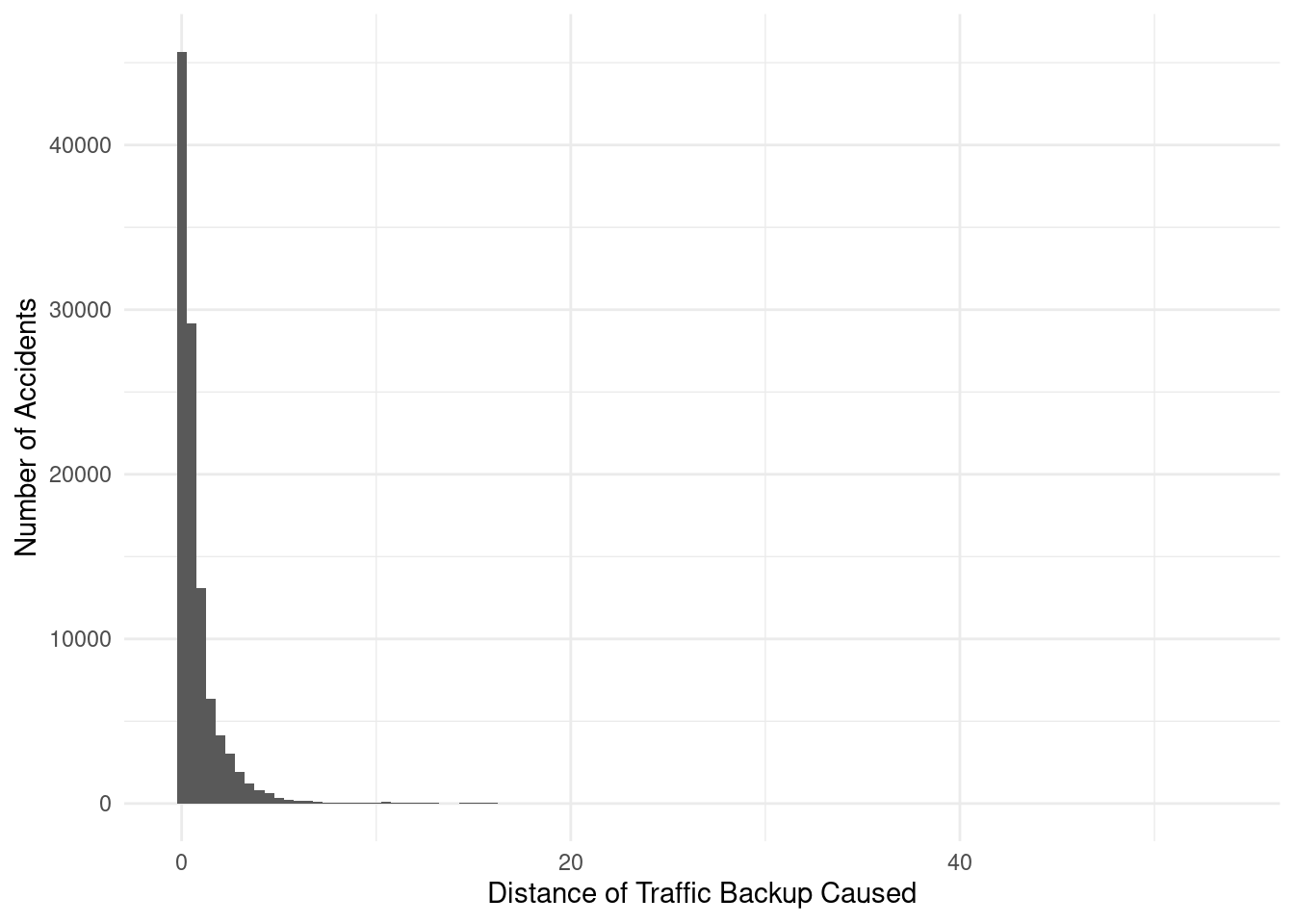
ggplot(data = nyacc, mapping = aes(x = Distance.mi.)) +
geom_histogram(binwidth = 0.5) +
theme_minimal() +
labs(
x = "Distance of Traffic Backup Caused",
y = "Number of Accidents",
Title = "Backup Lengths of Recorded Accidents"
)
nyacc |>
  ggplot(aes(x = Precipitation.in., y = Severity)) +
  geom_point() +
  labs(
    title = "Precipitation vs. Severity",
    x = "Precipitation (in)",
    y = "Severity"
  )
Warning: Removed 19660 rows containing missing values (`geom_point()`).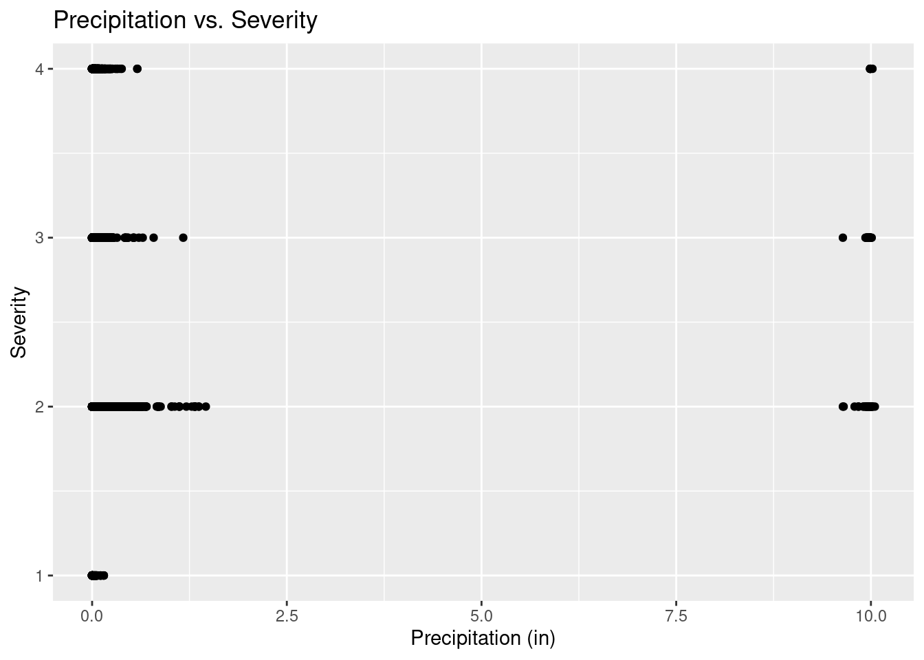
nyacc |>
  ggplot(aes(Severity, fill = Sunrise_Sunset)) +
  geom_histogram() +
  scale_color_viridis_d() +
  theme_minimal() +
  labs(
    title = "Time of Day vs. Severity",
    fill = "Time of Day"
  )
`stat_bin()` using `bins = 30`. Pick better value with `binwidth`.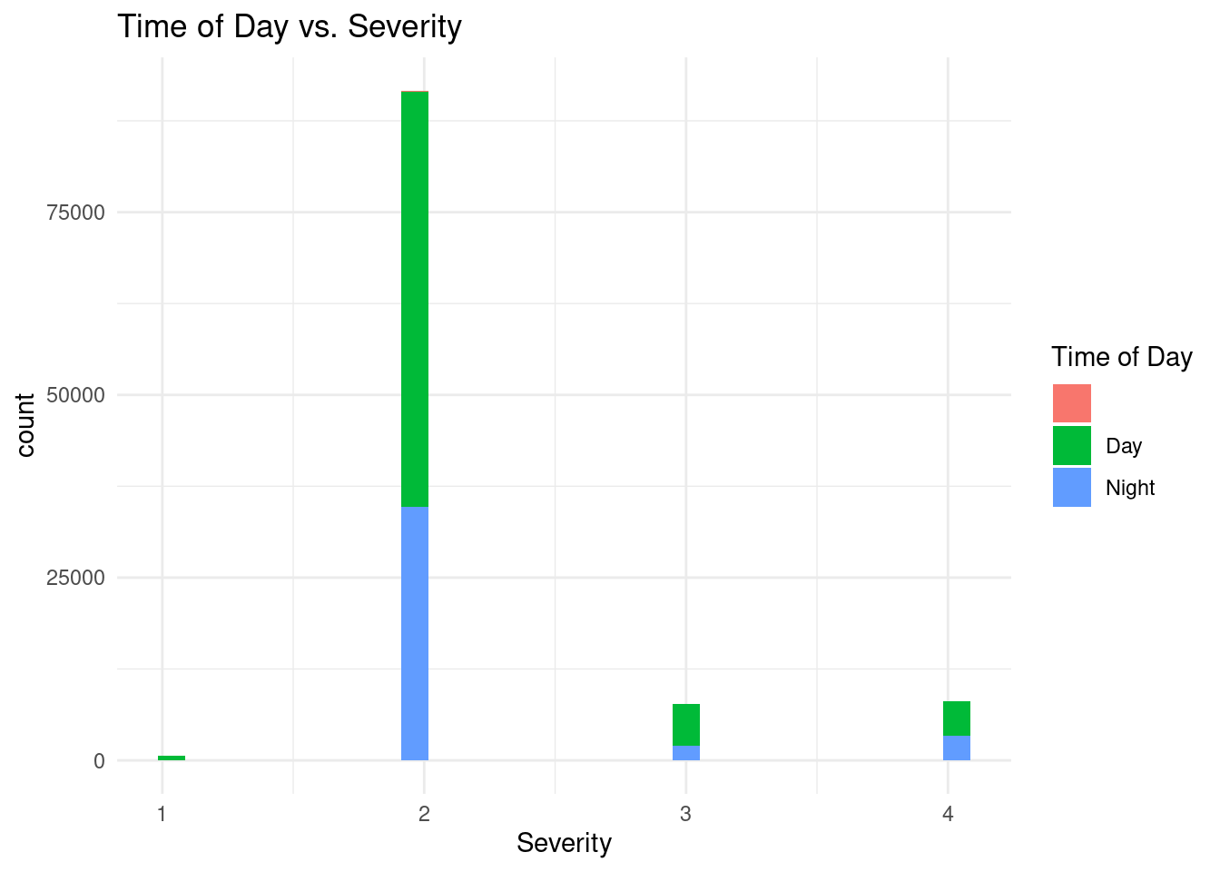
ggplot(nyacc, aes(x = Precipitation.in., fill = as.factor(Severity))) +
  geom_density(alpha = 0.5) +
  scale_x_sqrt() +
  labs(
    title = "Precipitation vs. Severity",
    x = "Precipitation (in)",
    fill = "Severity"
  )
Warning: Removed 19660 rows containing non-finite values (`stat_density()`).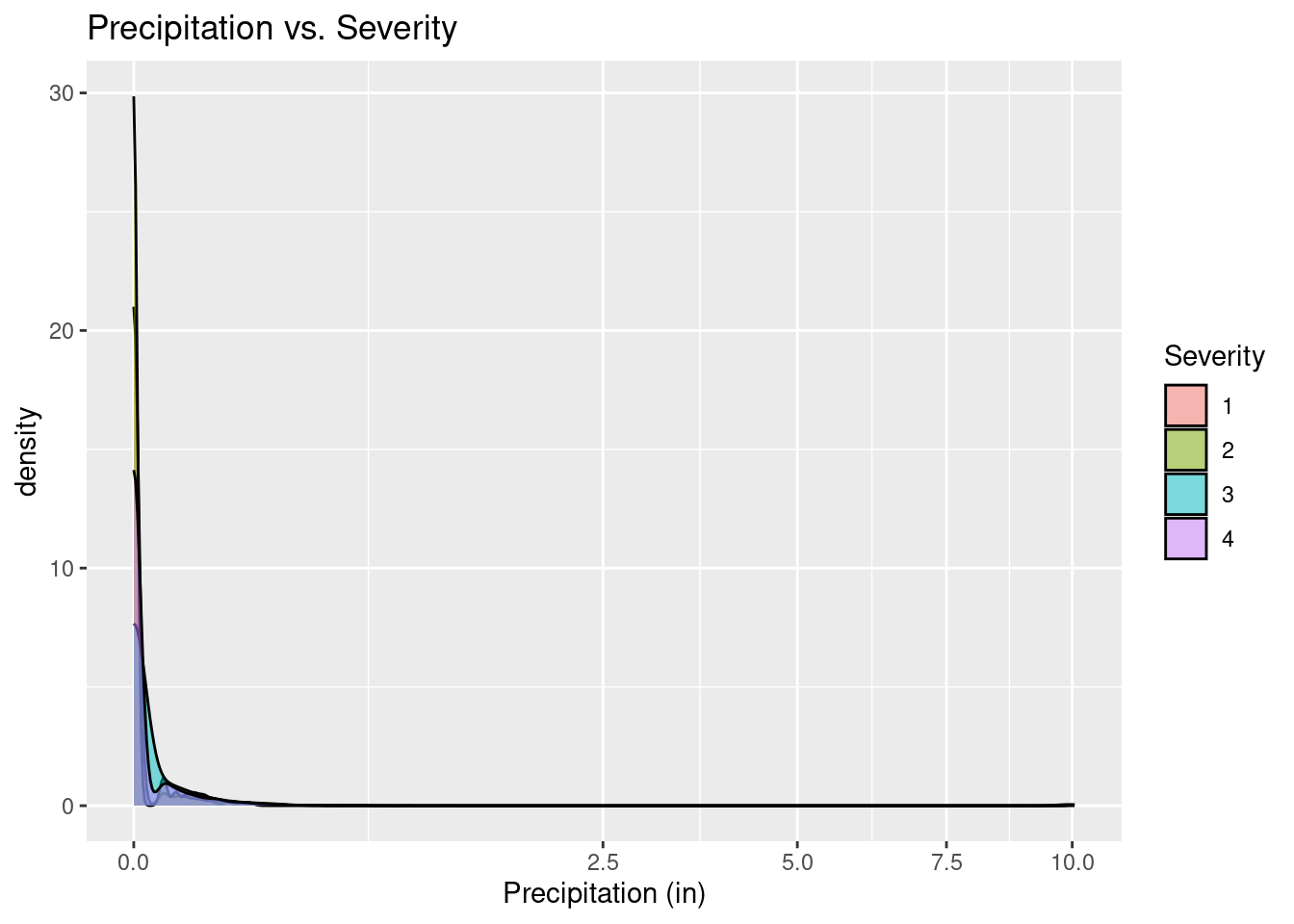
Logistic Regression
Our reason for doing logistic regression:
We are trying to find the probability that weather and/or time of day increase the severity of an accident.
# mutate data to more closely define how severe
severe <- c("3", "4")
not_severe <- c("1", "2")
relevant_weather <- c(
  "Clear", "Fog",
  "Snow", "T-Storm",
  "Rain", "Heavy Rain",
  "Heavy Snow"
)

# need to combine weathers

severity_weather_time <- nyacc |>
  select(Severity, Weather_Condition, Sunrise_Sunset) |>
  mutate(
    Severity = as.character(Severity),
    Severity = if_else(Severity %in% severe, "Very severe", Severity),
    Severity = if_else(Severity %in% not_severe, "Not too severe", Severity)
  ) |>
  filter(Weather_Condition %in% relevant_weather) |>
  arrange(desc(Weather_Condition)) |>
  na.omit()

# unique_weather <- nyacc |>
#  select(Weather_Condition) |>
#  count(Weather_Condition)

# unique_weather
# Analysis 1: Predicting severity from just weather condition
pred_severity_weather <- logistic_reg() |>
fit(as.factor(Severity) ~ Weather_Condition, data = severity_weather_time)
tidy(pred_severity_weather)# A tibble: 7 × 5
term estimate std.error statistic p.value
<chr> <dbl> <dbl> <dbl> <dbl>
1 (Intercept) -0.532 0.0289 -18.4 1.40e-75
2 Weather_ConditionFog -1.51 0.0904 -16.7 7.75e-63
3 Weather_ConditionHeavy Rain -1.20 0.135 -8.95 3.67e-19
4 Weather_ConditionHeavy Snow -1.13 0.189 -5.97 2.43e- 9
5 Weather_ConditionRain -1.35 0.0931 -14.5 6.41e-48
6 Weather_ConditionSnow -1.17 0.139 -8.42 3.71e-17
7 Weather_ConditionT-Storm -1.56 0.295 -5.27 1.35e- 7# Analysis 2: Predicting severity from just weather condition and time
pred_severity_weather_time <- logistic_reg() |>
fit(as.factor(Severity) ~ Weather_Condition + Sunrise_Sunset,
data = severity_weather_time
)
tidy(pred_severity_weather_time)# A tibble: 9 × 5
term estimate std.error statistic p.value
<chr> <dbl> <dbl> <dbl> <dbl>
1 (Intercept) 0.787 1.08 0.728 4.67e- 1
2 Weather_ConditionFog -1.59 0.0914 -17.4 1.82e-67
3 Weather_ConditionHeavy Rain -1.23 0.135 -9.10 9.07e-20
4 Weather_ConditionHeavy Snow -1.09 0.190 -5.77 8.11e- 9
5 Weather_ConditionRain -1.35 0.0933 -14.5 8.97e-48
6 Weather_ConditionSnow -1.16 0.139 -8.31 9.91e-17
7 Weather_ConditionT-Storm -1.56 0.297 -5.26 1.47e- 7
8 Sunrise_SunsetDay -1.43 1.08 -1.33 1.85e- 1
9 Sunrise_SunsetNight -1.10 1.08 -1.02 3.10e- 1# Analysis 1 prediction
ep_10 <- tibble(Weather_Condition = "Rain")
predict(pred_severity_weather, new_data = ep_10, type = "prob")# A tibble: 1 × 2
`.pred_Not too severe` `.pred_Very severe`
<dbl> <dbl>
1 0.868 0.132# Analysis 2 prediction
ep_10 <- tibble(Weather_Condition = "Rain", Sunrise_Sunset = "Night")
predict(pred_severity_weather_time, new_data = ep_10, type = "prob")# A tibble: 1 × 2
`.pred_Not too severe` `.pred_Very severe`
<dbl> <dbl>
1 0.841 0.159Resulting Equations from Logistic Regression:
\[ \begin{split} log(severity/(1-severity)) = -0.53 - 1.5 \times fog -1.2 \times heavy~rain - \\ 1.1 \times heavy~snow- 1.4 \times rain - \\ 1.2 \times snow -1.6 \times t~storm \end{split} \]
\[ \begin{split} log(severity/(1-severity)) = 0.8 - 1.6 \times fog - 1.2 \times heavy~rain - \\ 1.1 \times heavy~snow -1.4 \times rain - 1.2 \times snow - \\ 1.6 \times t~storm - 1.4 \times day - 1.1 \times night \end{split} \]
Explanation of Results:
For our logistic model with only weather conditions taken into account, the chance of the accident being very severe is 0.37 with no hazardous weather. If one of the tested weather features where present during the accident, the chance of being severe would decrease. The amount the chances would decrease for each weather condition ranging between 26.0% for a thunder storm and 21.1% for heavy snow. For accidents where there was rain, the model predicts that it will be very severe with probability 13.17%.
For our logistic model with weather conditions and time of day, the chance of it being severe is 68.7%. A clear evening would have a 42.3% chance of being severe. A Rainy Night would have a 15.9% chance of being severe. Each hazardous weather condition on its own would decrease the chance of severity by an amount ranging from 37.7 for fog to 26.3 for heavy snow.
The fact that more hazard driving conditions lessens the chance of severity is counterintuitive. It may be due to a flawed model that is a poor fit and does not describe the phenomena well, or there may be some possible explanation, such as in poor driving conditions, there are less people on the roads, so when an accident does occur, the backup is less severe. If it were true that delays are less in harsher conditions, investigating this could be an avenue for future research.
Evaluation of significance
Hypothesis Testing
Our reason for doing hypothesis testing:
We wish to test that the fact that severity of accidents increasing because of weather condition or time of day must be due to something other than chance.
Hypotheses:
Analysis 1:
Question: Do worse weather conditions (e.g. Light Rain vs. Heavy Rain, Light Snow, Heavy Snow, etc.) imply that accidents will be more severe in New York? We want to investigate the relationship between the severity of accidents and weather conditions in New York. Specifically, we are interested in how well the weather conditions on the day of the accident explains or predicts how severe the accident is.
Hypothesis:
\[ H_0: p_{heavy~snow} - p_{clear} = 0 \]
\[ H_A: p_{heavy~snow} - p_{clear} \neq 0 \]
Analysis 2:
Question:
- Does the time of day have an effect on the severity of the accident if it occurs during the night vs. day in New York? We want to analyze the relationship between at what time of the day accidents occur and the severity of accidents.
Hypothesis:
\[ H_0: p_{day} - p_{night} = 0 \]
\[ H_a: p_{day} - p_{night} \neq 0 \]
set.seed(123)
# Analysis 1: Predicting severity from weather condition
# keep severe vs not too severe
# if you have heavy snow, is it more likely to be severe than not severe?
# success = Very severe
# should filter to be just clear vs heavy snow
# changed up hypothesis because we accidentally wrote down the wrong variables
heavy_snow <- c("Clear", "Heavy Snow")

heavy_snow_pred <- severity_weather_time |>
  select(Severity, Weather_Condition) |>
  filter(Weather_Condition %in% heavy_snow)

null_weather <- heavy_snow_pred |>
  specify(response = Severity, explanatory = Weather_Condition, success = "Very severe") |>
  hypothesize(null = "independence") |>
  generate(1000, type = "permute") |>
  calculate(stat = "diff in props", order = c("Clear", "Heavy Snow"))

get_ci(x = null_weather, level = 0.9)
# A tibble: 1 × 2
lower_ci upper_ci
<dbl> <dbl>
1 -0.0535 0.0540point_estimate1 <- heavy_snow_pred |>
specify(response = Severity, explanatory = Weather_Condition, success = "Very severe") |>
calculate(stat = "diff in props", order = c("Clear", "Heavy Snow"))
get_p_value(x = null_weather, obs_stat = point_estimate1, direction = "two sided")Warning: Please be cautious in reporting a p-value of 0. This result is an
approximation based on the number of `reps` chosen in the `generate()` step. See
`?get_p_value()` for more information.# A tibble: 1 × 1
p_value
<dbl>
1 0visualize(null_weather) +
shade_p_value(obs_stat = point_estimate1, direction = "two sided")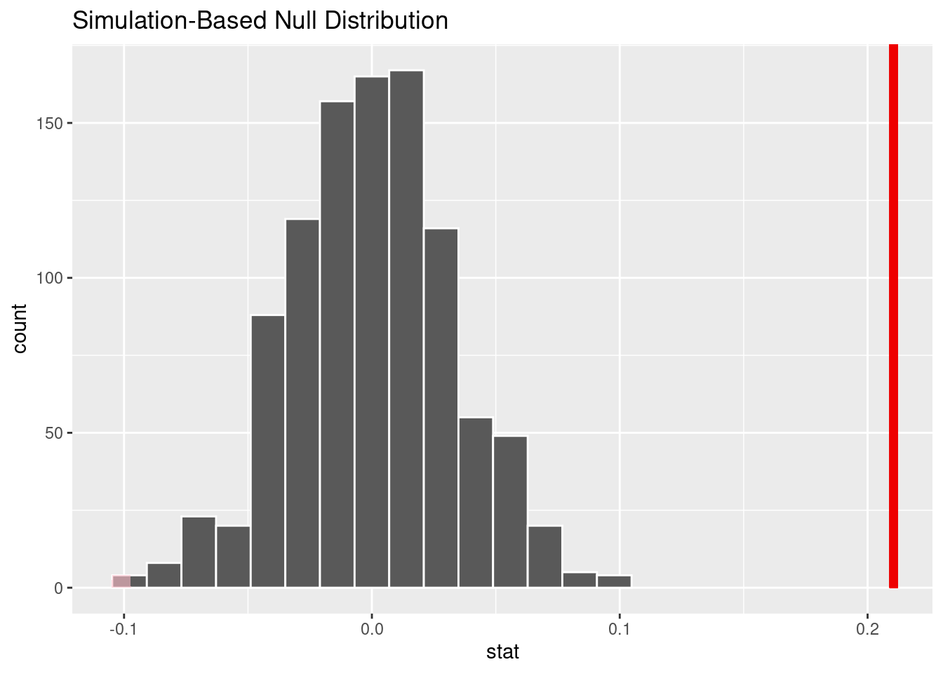
Conclusion of Analysis 1: Since our p-value is 0, which is less than 0.05, we reject the null hypothesis. We conclude that the weather condition of heavy snow does have an effect on the severity of an accident. It is also important to notice that our null distribution graph is showing a different p-value that our analysis is.
# Analysis 2: Predicting severity from time of day
valid_response <- c("Day", "Night")

time_pred <- severity_weather_time |>
  select(Severity, Sunrise_Sunset) |>
  filter(Sunrise_Sunset %in% valid_response)

null_time <- time_pred |>
  specify(response = Severity, explanatory = Sunrise_Sunset, success = "Very severe") |>
  hypothesize(null = "independence") |>
  generate(1000, type = "permute") |>
  calculate(stat = "diff in props", order = c("Day", "Night"))

get_ci(x = null_time, level = 0.9)
# A tibble: 1 × 2
lower_ci upper_ci
<dbl> <dbl>
1 -0.0170 0.0162point_estimate2 <- time_pred |>
specify(response = Severity, explanatory = Sunrise_Sunset, success = "Very severe") |>
calculate(stat = "diff in props", order = c("Day", "Night"))
get_p_value(x = null_time, obs_stat = point_estimate2, direction = "two sided")Warning: Please be cautious in reporting a p-value of 0. This result is an
approximation based on the number of `reps` chosen in the `generate()` step. See
`?get_p_value()` for more information.# A tibble: 1 × 1
p_value
<dbl>
1 0visualize(null_time) +
shade_p_value(obs_stat = point_estimate2, direction = "two sided")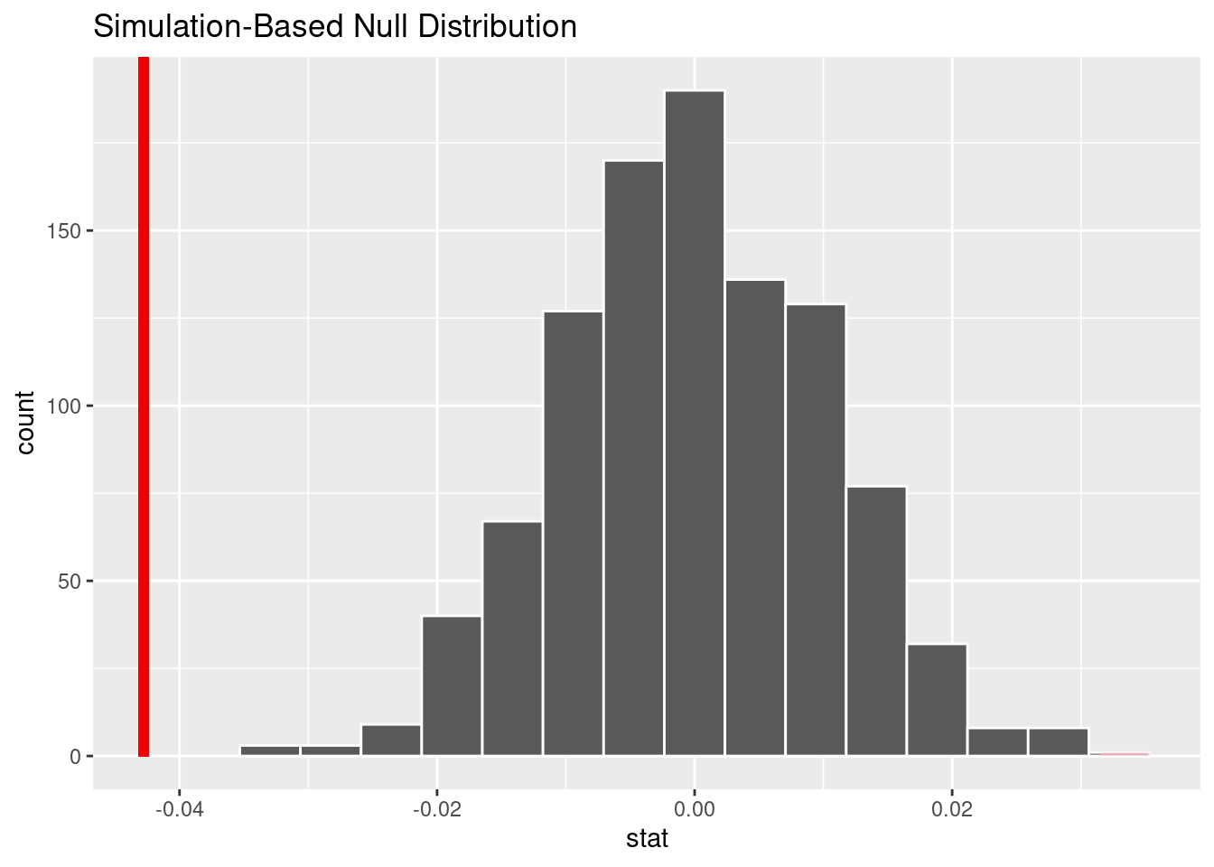
Conlusion of Analysis 2: Since our p-value is 0, which is less than 0.05, we reject the null hypothesis. We conclude that the time of day does have an effect on the severity of an accident.
Interpretation and conclusions
From our visual, we can see that the vast majority of accidents usually cause a backup of less than ½ of a mile. This may include accidents where the backup was only a block or so, or accidents where there was no backup. For the context of predicting delays to drivers, this may mean that there are often not long areas of delay. However, this cannot be seen as that there are often no delays, as a half mile backup would cause a significant delay despite a short distance.
Our other visuals showing the relationship between precipitation and severity or time of day and severity show that there is not much clearly evident linear relationship between precipitation and severity or time of day and severity.
Interpretations of Log Results:
From our log odds equation, log(p/1-p) of model 1, we determine that an accident without any of the investigated weather conditions has odds of -0.53 of being not severe. Having just one of the conditions lowers the chance that it is not severe to 16.2%-30.2%. From our log odds equation, log(p/1-p) of model 2, we determine that an accident without any of the investigated weather conditions has odds of 0.78 of being not severe. Having just one of the conditions lowers the chance that it is not severe to 16.2%-30.2%.
Interpretation of Hypothesis Tests:
Since both of our hypothesis tests had the result of the p-value being 0, we can conclude that weather condition of heavy snow does have an effect on the severity of an accident and that the time of day does have an effect on the severity of an accident.
Limitations
Though our dataset is incredibly comprehensive and in depth with 1.5 million accident records, its limitations lie in the fact that its data collection began in only 2016 and covers only 49 states. The data contains variables concerning things such as location, severity, time, weather, and type of accident. However, there are 5 ways to find the time of the accident. Though this allows the dataset to be comprehensive and cover the different ways people measure time, it is confusing to the analyzer and can cause the dataset to be redundant. In addition, some variables are left quite vague such as severity which is only a 1-4 level basis with 1 being least impact on traffic and 4 being significant impact on traffic. However, this severity can be measured through various factors and can be changed by factors that are being used in the specific scale. It is also important to acknowledge the fact that this dataset does not account for every single accident that has happened in New York because there are many accidents left unreported or even manipulated.
It gives us many unique metrics to understand the different details and nuances of the accident, which are incredibly helpful to visualize the complexity of the situation. The data contains variables concerning things such as location, severity, time, weather, and type of accident, which are all detailed and standardized in its presentation format. It contains details on over 1.5 million accident records and contains data from 2016 onwards from 49 states.
Acknowledgments
We would like to acknowledge Sobhan Moosavi who worked on this US-Accidents: A Countrywide Traffic Accident Dataset. He has published an in-depth description of the dataset and its variables that has helped us understand the dataset. Here is the link: https://smoosavi.org/datasets/us_accidents.