Attaching package: 'janitor'

The following objects are masked from 'package:stats':

    chisq.test, fisher.test
Research question(s)
We aim to discover the relationship between certain characteristics of the exoneree and their case and the type of sentence that they received. More specifically, we want to know how race, age at time of the crime, sex, the time they spent before being exonerated, and the important details that led to their exoneration (perjury, inadequate legal defense, etc.) relate to the severity of their sentence.
Using this analysis, we hope to be able to use these variables to predict the severity of their sentence.
Data collection and cleaning
Have an initial draft of your data cleaning appendix. Document every step that takes your raw data file(s) and turns it into the analysis-ready data set that you would submit with your final project. Include text narrative describing your data collection (downloading, scraping, surveys, etc) and any additional data curation/cleaning (merging data frames, filtering, transformations of variables, etc). Include code for data curation/cleaning, but not collection.
First, we request and download the raw .csv file from the National Registry of Exonerations.
Rows: 3284 Columns: 23
── Column specification ────────────────────────────────────────────────────────
Delimiter: ","
chr (20): Last Name, First Name, Race, Sex, State, County, Tags, Worst Crime...
dbl  (3): Age, Convicted, Exonerated

ℹ Use `spec()` to retrieve the full column specification for this data.
ℹ Specify the column types or set `show_col_types = FALSE` to quiet this message.
The dataset is already generally clean and tidy, with each row representing a exoneree and the various details of their case. However, there are some improvements to be made. First is the column names, which do not follow convention and include several strange characters in them. We use the janitor function clean_names to give the names a proper format.
Next, we want to transform the tags column so we can use its contents for further analysis. Originally, these tags were contained in a “;#” separated string. To pull them out, we mutate our dataframe to include a new column that indicates whether or not the exoneree’s case included that tag.
Several of the columns had values of NA or the name of the column itself to demonstrate a binary set of values. We convert these to simply 1 and 0 for ease of analysis.
Next, we create a new column that represents the number of years between when an exoneree was convicted and when they were exonerated. This gives us an estimate of how long they spent in prison, on probation, or, more generally, faced the consequences of a crime they did not commit. We also add a column sentence_severity, which marks whether or not the exoneree was sentenced to a severe punishment (death, life in prison, or life without parole). These will aid us in our analysis later.
Finally, we filter out the columns that we will not be using in our analysis or have already used in different forms (i.e. tags column).
most_severe <-c("Death", "Life without parole", "Life")# turn tags into columns, mark 1 if tag present, 0 if notus_exonerations <- us_exonerations |>clean_names() |>rowwise() |>mutate(tags_vc =str_split(string = tags, pattern =";#"),ars =if_else("A"%in% tags_vc, 1, 0),cdc =if_else("CDC"%in% tags_vc, 1, 0),ciu =if_else("CIU"%in% tags_vc, 1, 0),csh =if_else("CSH"%in% tags_vc, 1, 0),cv =if_else("CV"%in% tags_vc, 1, 0),fem =if_else("F"%in% tags_vc, 1, 0),fed =if_else("FED"%in% tags_vc, 1, 0),hom =if_else("H"%in% tags_vc, 1, 0),ji =if_else("JI"%in% tags_vc, 1, 0),m =if_else("M"%in% tags_vc, 1, 0),nc =if_else("NC"%in% tags_vc, 1, 0),p =if_else("P"%in% tags_vc, 1, 0),ph =if_else("PH"%in% tags_vc, 1, 0),sbs =if_else("SBS"%in% tags_vc, 1, 0),sa =if_else("SA"%in% tags_vc, 1, 0) ) |>ungroup() |>mutate(dna =if_else(is.na(dna), 0, 1),fc =if_else(is.na(fc), 0, 1),mwid =if_else(is.na(mwid), 0, 1),f_mfe =if_else(is.na(f_mfe), 0, 1),p_fa =if_else(is.na(p_fa), 0, 1),om =if_else(is.na(om), 0, 1),ild =if_else(is.na(ild), 0, 1),# calculate the number of years between conviction and exonerationdiff_conv_ex = exonerated - convicted,# column that designates whether or not they had the highest severity punishmentsentence_severity =if_else(sentence %in% most_severe, "Yes", "No") ) |>select(-om_tags, -tags_vc, -list_addl_crimes_recode, -tags, -x)us_exonerations
# A tibble: 3,284 × 36
   last_name first_name     age race     sex    state county worst_crime_display
   <chr>     <chr>        <dbl> <chr>    <chr>  <chr> <chr>  <chr>
 1 Abbitt    Joseph          31 Black    Male   Nort… Forsy… Child Sex Abuse
 2 Abbott    Cinque          19 Black    Male   Illi… Cook   Drug Possession or…
 3 Abdal     Warith Habib    43 Black    Male   New … Erie   Sexual Assault
 4 Abernathy Christopher     17 White    Male   Illi… Cook   Murder
 5 Abney     Quentin         32 Black    Male   New … New Y… Robbery
 6 Abrego    Eruby           20 Hispanic Male   Illi… Cook   Murder
 7 Acero     Longino         35 Hispanic Male   Cali… Santa… Sex Offender Regis…
 8 Adams     Anthony         26 Hispanic Male   Cali… Los A… Manslaughter
 9 Adams     Cheryl          26 White    Female Mass… Essex  Theft
10 Adams     Darryl          25 Black    Male   Texas Dallas Sexual Assault
# ℹ 3,274 more rows
# ℹ 28 more variables: sentence <chr>, convicted <dbl>, exonerated <dbl>,
#   dna <dbl>, fc <dbl>, mwid <dbl>, f_mfe <dbl>, p_fa <dbl>, om <dbl>,
#   ild <dbl>, posting_date <chr>, ars <dbl>, cdc <dbl>, ciu <dbl>, csh <dbl>,
#   cv <dbl>, fem <dbl>, fed <dbl>, hom <dbl>, ji <dbl>, m <dbl>, nc <dbl>,
#   p <dbl>, ph <dbl>, sbs <dbl>, sa <dbl>, diff_conv_ex <dbl>,
#   sentence_severity <chr>
skimr::skim(us_exonerations)
Data summary
Name
us_exonerations
Number of rows
3284
Number of columns
36
_______________________
Column type frequency:
character
10
numeric
26
________________________
Group variables
None
Variable type: character
skim_variable
n_missing
complete_rate
min
max
empty
n_unique
whitespace
last_name
0
1.00
2
18
0
2034
0
first_name
0
1.00
2
18
0
1305
0
race
0
1.00
5
22
0
9
0
sex
0
1.00
4
6
0
2
0
state
0
1.00
4
20
0
84
0
county
60
0.98
3
17
0
568
0
worst_crime_display
0
1.00
5
29
0
45
0
sentence
0
1.00
2
45
0
480
0
posting_date
0
1.00
8
10
0
1230
0
sentence_severity
0
1.00
2
3
0
2
0
Variable type: numeric
skim_variable
n_missing
complete_rate
mean
sd
p0
p25
p50
p75
p100
hist
age
26
0.99
28.43
10.24
11
20
26
34
83
▇▆▂▁▁
convicted
0
1.00
1998.64
10.97
1956
1990
1998
2007
2021
▁▁▇▇▅
exonerated
0
1.00
2010.45
8.96
1989
2003
2013
2018
2023
▂▃▅▇▇
dna
0
1.00
0.17
0.38
0
0
0
0
1
▇▁▁▁▂
fc
0
1.00
0.12
0.33
0
0
0
0
1
▇▁▁▁▁
mwid
0
1.00
0.27
0.44
0
0
0
1
1
▇▁▁▁▃
f_mfe
0
1.00
0.24
0.42
0
0
0
0
1
▇▁▁▁▂
p_fa
0
1.00
0.63
0.48
0
0
1
1
1
▅▁▁▁▇
om
0
1.00
0.59
0.49
0
0
1
1
1
▆▁▁▁▇
ild
0
1.00
0.27
0.44
0
0
0
1
1
▇▁▁▁▃
ars
0
1.00
0.03
0.16
0
0
0
0
1
▇▁▁▁▁
cdc
0
1.00
0.13
0.34
0
0
0
0
1
▇▁▁▁▁
ciu
0
1.00
0.20
0.40
0
0
0
0
1
▇▁▁▁▂
csh
0
1.00
0.02
0.13
0
0
0
0
1
▇▁▁▁▁
cv
0
1.00
0.20
0.40
0
0
0
0
1
▇▁▁▁▂
fem
0
1.00
0.09
0.28
0
0
0
0
1
▇▁▁▁▁
fed
0
1.00
0.04
0.20
0
0
0
0
1
▇▁▁▁▁
hom
0
1.00
0.39
0.49
0
0
0
1
1
▇▁▁▁▅
ji
0
1.00
0.07
0.25
0
0
0
0
1
▇▁▁▁▁
m
0
1.00
0.03
0.18
0
0
0
0
1
▇▁▁▁▁
nc
0
1.00
0.40
0.49
0
0
0
1
1
▇▁▁▁▆
p
0
1.00
0.24
0.43
0
0
0
0
1
▇▁▁▁▂
ph
0
1.00
0.01
0.09
0
0
0
0
1
▇▁▁▁▁
sbs
0
1.00
0.01
0.10
0
0
0
0
1
▇▁▁▁▁
sa
0
1.00
0.27
0.44
0
0
0
1
1
▇▁▁▁▃
diff_conv_ex
0
1.00
11.80
9.84
0
4
9
18
58
▇▅▂▁▁
Data description
Have an initial draft of your data description section. Your data description should be about your analysis-ready data.
The US exonerations data is from the National Registry of Exonerations. This is funded by University of Michigan, Michigan State University, and University of California Irvine. There are 26 columns and 3.2K rows. This data set contains all of the exonerations in the US since 1989. The rows are each individual who was exonerated of their crime, meaning that they were wrongfully found guilty but in the end found innocent on all crimes. The columns are the information about the individual, such as how long they were in jail, their race, name, age, state, and crime. The registry gets their data from the courts and government agencies, so it contains all of the known exonerations. The National Registry of Exonerations’ goal is to change the criminal justice system by highlighting the amount of exonerations there are and making individuals more aware.
Data limitations
Because this dataset is constantly being updated, there are some inconsistencies with the data and the provided codebook. For example, there are tags that exist in our data but not in the codebook. Further, there are some issue with inconsistencies in how data has been entered into the database, particularly in the lack of a standardized format for the sentencing. There is also a question of how accurate the data is, given that they are reporting on exoneration cases more than 30 years ago.
Another limitation about this data set is the amount of observations. Although there are several thousand in total, when we start to try to analyze subgroups we may run into the issue of having too few observations.
Exploratory data analysis
Perform an (initial) exploratory data analysis.
First, to get a general sense of the dataset, we look at some basic summary statistics for variables of interest.
# proportion of males to femalesus_exonerations |>group_by(sex) |>summarize(num =n() ) |>ungroup() |>mutate(prop = num /sum(num) )
# A tibble: 2 × 3
  sex      num   prop
  <chr>  <int>  <dbl>
1 Female   284 0.0865
2 Male    3000 0.914
# proportion of exonerees by raceus_exonerations |>group_by(race) |>summarize(num =n() ) |>ungroup() |>mutate(prop = num /sum(num) )
# A tibble: 9 × 3
  race                     num     prop
  <chr>                  <int>    <dbl>
1 Asian                     32 0.00974
2 Black                   1724 0.525
3 Black;#White               1 0.000305
4 Don't Know                 7 0.00213
5 Hispanic                 400 0.122
6 Native American           22 0.00670
7 Native American;#White     1 0.000305
8 Other                     19 0.00579
9 White                   1078 0.328
# in how many cases was DNA evidence a significant portion of the exoneration case?us_exonerations |>summarize(dna_sum =sum(dna) )
# A tibble: 1 × 1
  dna_sum
    <dbl>
1     574
# on average, how long were exonerees convicted for before their exoneration?us_exonerations |>summarize(mean_exon =mean(diff_conv_ex) )
# A tibble: 1 × 1
  mean_exon
      <dbl>
1      11.8
# what is the distribution of exoneration case evidence (DNA, perjury, false confession, etc.)us_exonerations |>summarize(dna_sum =sum(dna),fc_sum =sum(fc),mwid_sum =sum(mwid),fmfe_sum =sum(f_mfe),pfa_sum =sum(p_fa),om_sum =sum(om),ild_sum =sum(ild) )
# what proportion of people receive a severe sentence>us_exonerations |>group_by(sentence_severity) |>summarize(num =n() ) |>ungroup() |>mutate (prop = num /sum(num) )
# A tibble: 2 × 3
  sentence_severity   num  prop
  <chr>             <int> <dbl>
1 No                 2423 0.738
2 Yes                 861 0.262
Next, we look at some visualizations for some potentially important relationships.
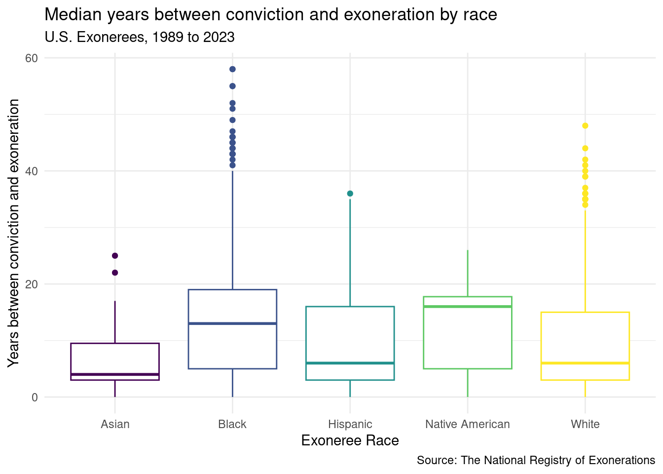
# box plot to show median length between conviction and exoneration by race# for visualization purposes, we consider only 5 races, Asian, Hispanic, Black, White, and Native Americanrace_5 <-c('Asian', 'Hispanic', 'Black', 'White', 'Native American')us_exonerations |>filter(race %in% race_5) |>ggplot(aes(x = race, y = diff_conv_ex, color = race)) +geom_boxplot(show.legend =FALSE) +scale_color_viridis_d() +labs(title ="Median years between conviction and exoneration by race",subtitle ="U.S. Exonerees, 1989 to 2023",x ="Exoneree Race",y ="Years between conviction and exoneration",caption ="Source: The National Registry of Exonerations" ) +theme_minimal()
This plot raises some interesting questions regarding race and time between years between conviction and exoneration as we can see some differences in the medians between the races. Is there some relationship between these two factors? If so, how might this interact with the severity of the sentence? We examine part of this idea in the next visualization.
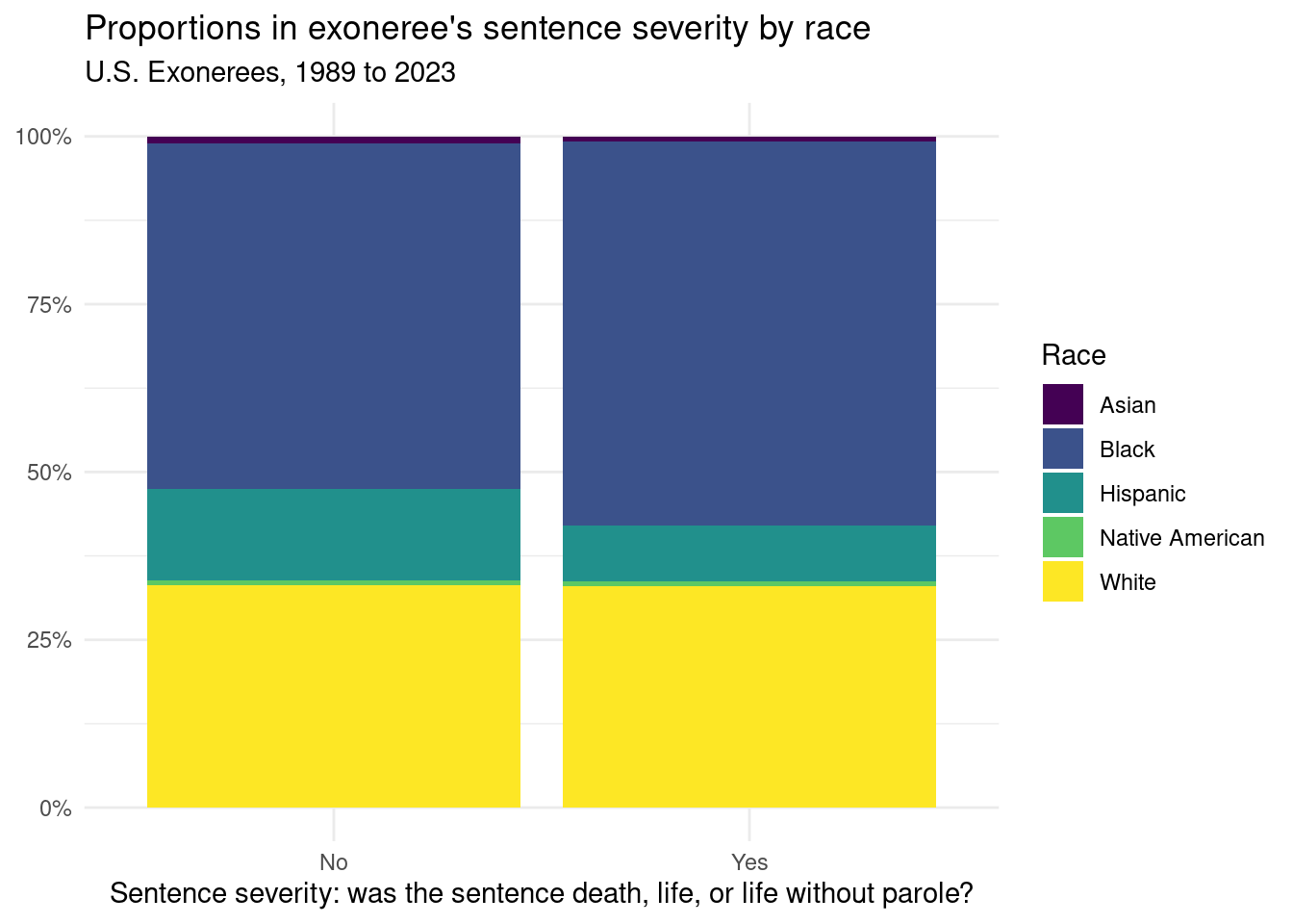
us_exonerations |>filter(race %in% race_5) |>ggplot(aes(x = sentence_severity, fill = race)) +geom_bar(position ="fill") +scale_fill_viridis_d() +scale_y_continuous(labels = scales::percent) +labs(title ="Proportions in exoneree's sentence severity by race",subtitle ="U.S. Exonerees, 1989 to 2023",x ="Sentence severity: was the sentence death, life, or life without parole?",y =NULL,fill ="Race" ) +theme_minimal()
In this plot, we aim to show the breakdown of sentence severity by race. Does race on its own play a role in determining how severe the sentence that exonerees get? We will need further analyses to answer this question.
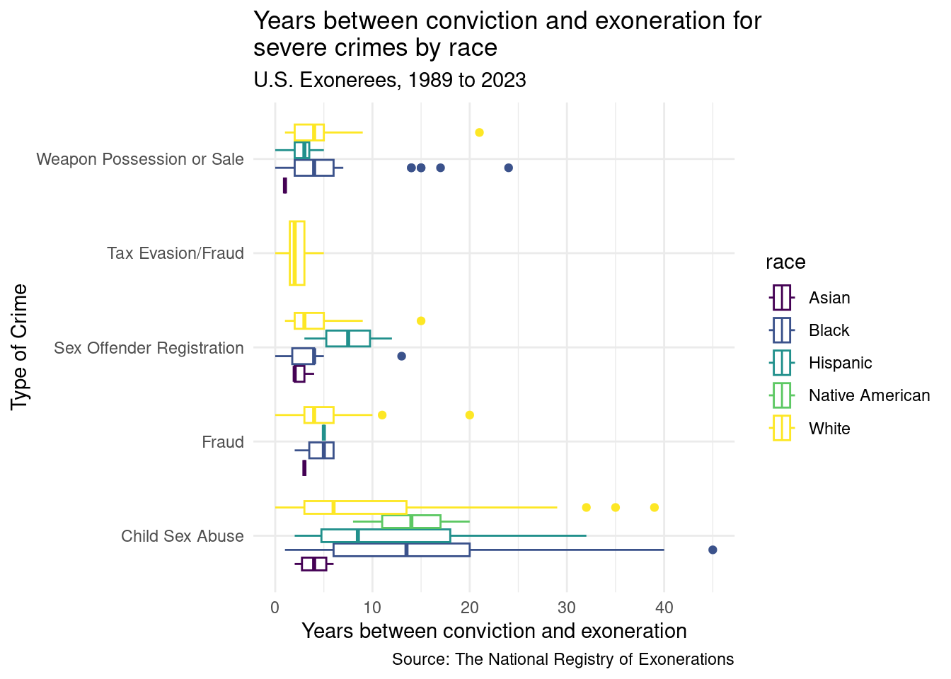
crime_5 <-c('Sex Offender Registration', 'Tax Evasion/Fraud', 'Weapon Possession or Sale', 'Fraud', 'Child Sex Abuse')us_exonerations |>filter(race %in% race_5, worst_crime_display %in% crime_5) |>ggplot(aes(x = diff_conv_ex, y = worst_crime_display, color = race)) +geom_boxplot() +scale_color_viridis_d() +labs(title ="Years between conviction and exoneration for\nsevere crimes by race",subtitle ="U.S. Exonerees, 1989 to 2023",x ="Years between conviction and exoneration",y ="Type of Crime",caption ="Source: The National Registry of Exonerations" ) +theme_minimal()
In this plot, we breakdown the relationship between the type of crime and the years between conviction and exoneration by race. What crimes have the greatest time between conviction and exoneration? How does race compare to the results for each crime?
Can we draw parallels between the severity of the crime and the severity of the sentence? How does race, or other factors, play a role in changing this relationship? These are questions that we would hope to answer with more analyses.
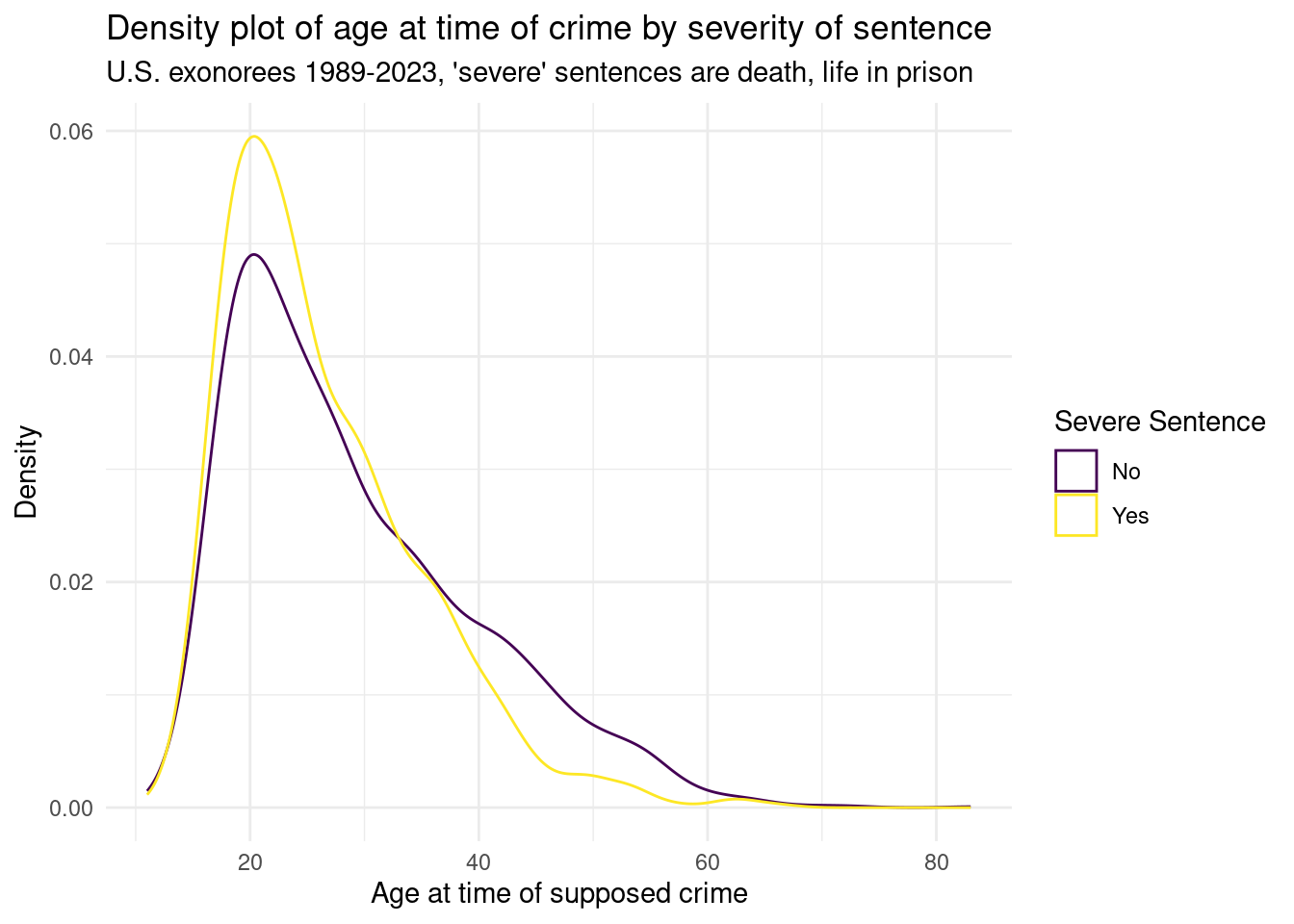
Another facet we can look at is the age at the time of the crime.
us_exonerations |>ggplot(aes(x = age, color = sentence_severity)) +geom_density() +scale_color_viridis_d() +theme_minimal() +labs(title ="Density plot of age at time of crime by severity of sentence",subtitle ="U.S. exonorees 1989-2023, 'severe' sentences are death, life in prison",x ="Age at time of supposed crime",y ="Density",color ="Severe Sentence" )
Interestingly, we can see that the distributions look very similar. Both severe sentence exonerees and other exonerees have a peak around 20.
Questions for reviewers
List specific questions for your peer reviewers and project mentor to answer in giving you feedback on this phase.
We would appreciate feedback to our research question: do you think the scope is clear and challenging enough for the purpose of this project?
We would also like feedback on our explorations: do they answer our research question and did we make the right choices in which data visualization we used?