Research question(s). State your research question (s) clearly.
Coffee is one of the most widely consumed beverages around the world, and with the current day world being more interconnected as ever, we have access to a vast variety of coffee beans from different places around the world that each differ slightly contributing to a different flavor. By researching into these geographical differences and analyzing the factors that contribute to the different flavors, consumers would be able to learn more about the different options and how the flavors differ such as in acidity, sweetness, fragrance, and balance to make their optimal choice. As we expect geographical location to be a main factor in affecting the taste of coffee, we expect that coffee beans from the same regions and altitudes would have similar ratings while coffee from differing regions and altitudes would have a greater difference in taste. Our research question explores how the countries and altitude of the coffee beans affect the rating of different coffees.
Data collection and cleaning
Have an initial draft of your data-cleaning appendix. Document every step that takes your raw data file(s) and turns it into the analysis-ready data set that you would submit with your final project. Include text narrative describing your data collection (downloading, scraping, surveys, etc) and any additional data curation/cleaning (merging data frames, filtering, transformations of variables, etc). Include code for data curation/cleaning, but not collection.
Rows: 1339 Columns: 43
── Column specification ────────────────────────────────────────────────────────
Delimiter: ","
chr (24): species, owner, country_of_origin, farm_name, lot_number, mill, ic...
dbl (19): total_cup_points, number_of_bags, aroma, flavor, aftertaste, acidi...

ℹ Use `spec()` to retrieve the full column specification for this data.
ℹ Specify the column types or set `show_col_types = FALSE` to quiet this message.
Warning: 9 parsing failures.
row col expected                actual
 14  -- a number May-August
316  -- a number January Through April
383  -- a number August to December
392  -- a number Mayo a Julio
424  -- a number Abril - Julio
... ... ........ .....................
See problems(...) for more details.
In order to clean the data, we got rid of unnecessary columns that we do not need in our investigation. The columns we kept in the data frames, such as country_of_origin, harvest_year, and aroma, all contribute relevant information to our study. Additionally, we further cleaned our data by dropping NULL values in each cell. Then, we cleaned up the harvest_year and grading_year by separating date, month, and year, leaving only the year of that specific coffee entry. Data cleaning can effectively help us to work with data more easily when we plot out graphs and explore relationships.
Data description
Have an initial draft of your data description section. Your data description should be about your analysis-ready data.
With the cleaned data, each observation contain information about a coffee bean (Arabica and Robusta) and its total cup points, species, country of origin, region, harvest year, grading year, aroma, flavor, aftertaste, acidity, body, balance, and altitude mean meters. The attributes and columns are the categories that the observation contains information about including total cup points, species, country of origin, region, harvest year, grading year, aroma, flavor, aftertaste, acidity, body, balance, and altitude mean meters. The original data set was funded by the Coffee Quality Institute and created by Buzzfeed Data Scientist James LeDoux to analyze the reviews of 1312 arabica and 28 robusta coffee beans and produce an article on the top coffee around the world. The process of James LeDoux using an external data set meant that the data was not directly observed and recorded by LeDoux so we do not know how the initial data was cleaned and chosen to be recorded or not. The data was first collected by having the Coffee Quality Institute’s trained reviewers do the reviews of the coffee beans. Then, James LeDoux analyzed the reviews and processed it into the current data form. The people involved were the Coffee Quality Institute’s trained reviewers and they were aware of the data collection and expected for their reviews/ ratings to be used for consumers to know about the flavor ratings of different coffees.
Data limitations
Identify any potential problems with your dataset.
A potential limiation of the dataset is that it only contains attributes/columns on flavor very vaguely in that we can only identify the flavor, aftertaste, aroma, acidity, body, and balance but will not be able to determine suppose if the coffee has a more sour flavor or bitter flavor.All the flavors are rated on the numerical scale and flavor is usually a preference thing for users so the numerical scales only a reflection of the reviewers’ taste.
Exploratory data analysis
Perform an (initial) exploratory data analysis.
skimr::skim(coffee_ratings_clean)
Data summary
Name
coffee_ratings_clean
Number of rows
1068
Number of columns
14
_______________________
Column type frequency:
character
4
numeric
10
________________________
Group variables
None
Variable type: character
skim_variable
n_missing
complete_rate
min
max
empty
n_unique
whitespace
species
0
1.00
7
7
0
2
0
country_of_origin
0
1.00
4
28
0
35
0
region
0
1.00
2
71
0
331
0
processing_method
64
0.94
5
25
0
5
0
Variable type: numeric
skim_variable
n_missing
complete_rate
mean
sd
p0
p25
p50
p75
p100
hist
total_cup_points
0
1
82.09
3.64
0
81.17
82.50
83.58
90.58
▁▁▁▁▇
harvest_year
0
1
2013.66
1.73
2009
2012.00
2014.00
2015.00
2018.00
▁▆▇▅▂
grading_year
0
1
2013.91
1.78
2010
2012.00
2014.00
2015.00
2018.00
▁▇▅▆▂
aroma
0
1
7.57
0.38
0
7.42
7.58
7.75
8.75
▁▁▁▁▇
flavor
0
1
7.52
0.40
0
7.33
7.50
7.75
8.83
▁▁▁▁▇
aftertaste
0
1
7.39
0.41
0
7.25
7.42
7.58
8.67
▁▁▁▁▇
acidity
0
1
7.53
0.39
0
7.33
7.50
7.75
8.75
▁▁▁▁▇
body
0
1
7.51
0.37
0
7.33
7.50
7.67
8.58
▁▁▁▁▇
balance
0
1
7.50
0.42
0
7.33
7.50
7.67
8.75
▁▁▁▁▇
altitude_mean_meters
0
1
1786.21
8833.03
1
1100.00
1310.64
1600.00
190164.00
▇▁▁▁▁
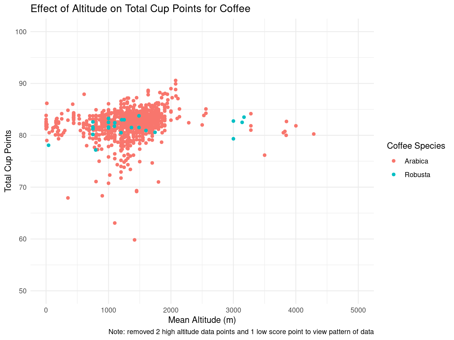
coffee_ratings_clean |>ggplot(mapping =aes(x = altitude_mean_meters, y = total_cup_points, color = species)) +geom_point() +labs(x ="Mean Altitude (m)",y ="Total Cup Points",title ="Effect of Altitude on Total Cup Points for Coffee",color ="Coffee Species",caption ="Note: removed 2 high altitude data points and 1 low score point to view pattern of data" ) +scale_x_continuous(limits =c(0, 5000)) +scale_y_continuous(limits =c(50, 100)) +theme_minimal()
We could not notice any particular pattern in the total cup points for each coffee type based on mean altitude (in meters). We decided to take a deeper look at each of the factors that affected the total cup points to see if there were any underlying trends.
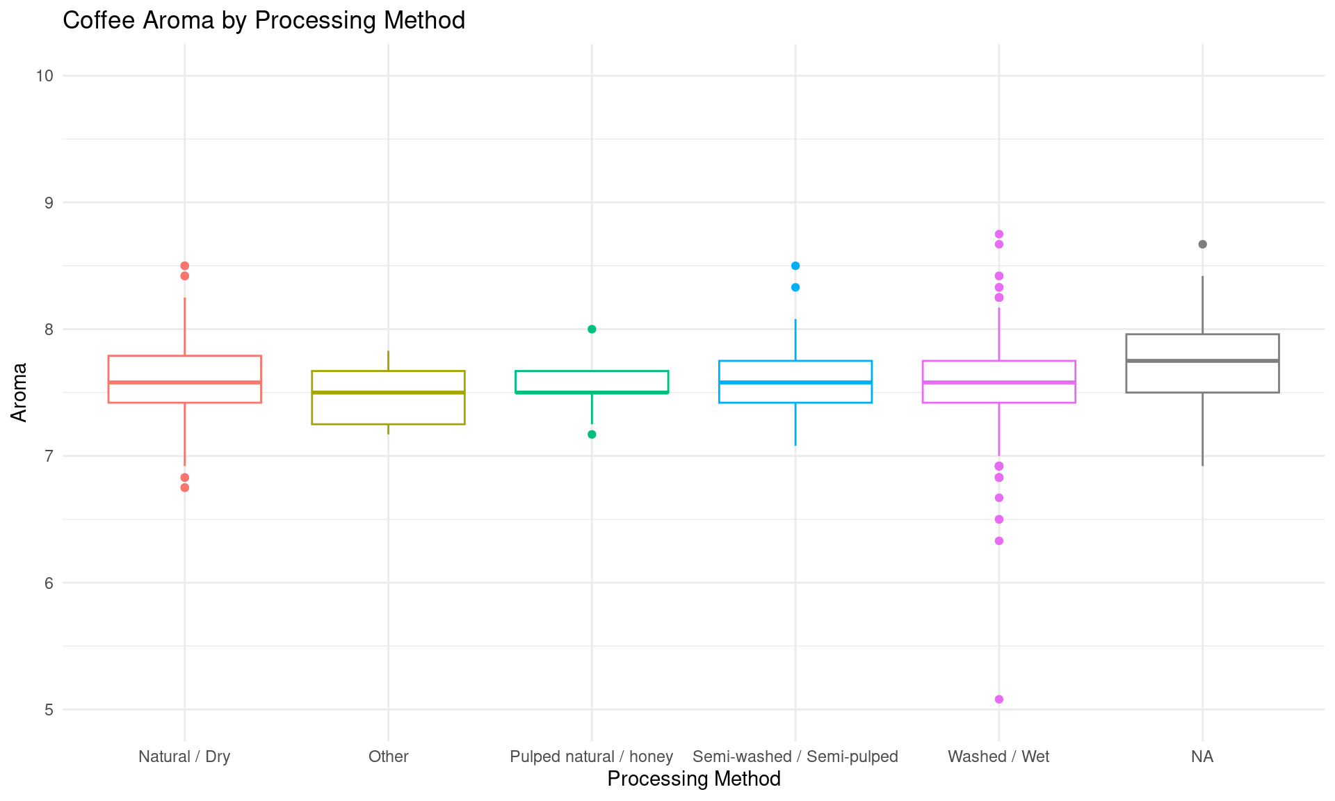
coffee_ratings_clean |>ggplot(mapping =aes(x = altitude_mean_meters, y = aroma, color = species)) +geom_point() +labs(x ="Mean Altitude (m)",y ="Aroma Score",title ="Effect of Altitude on Coffee Aroma",color ="Coffee Species",caption ="Note: removed 2 high altitude data points and 1 low score point to view pattern of data" ) +scale_x_continuous(limits =c(0, 5000)) +scale_y_continuous(limits =c(5, 10)) +theme_minimal()
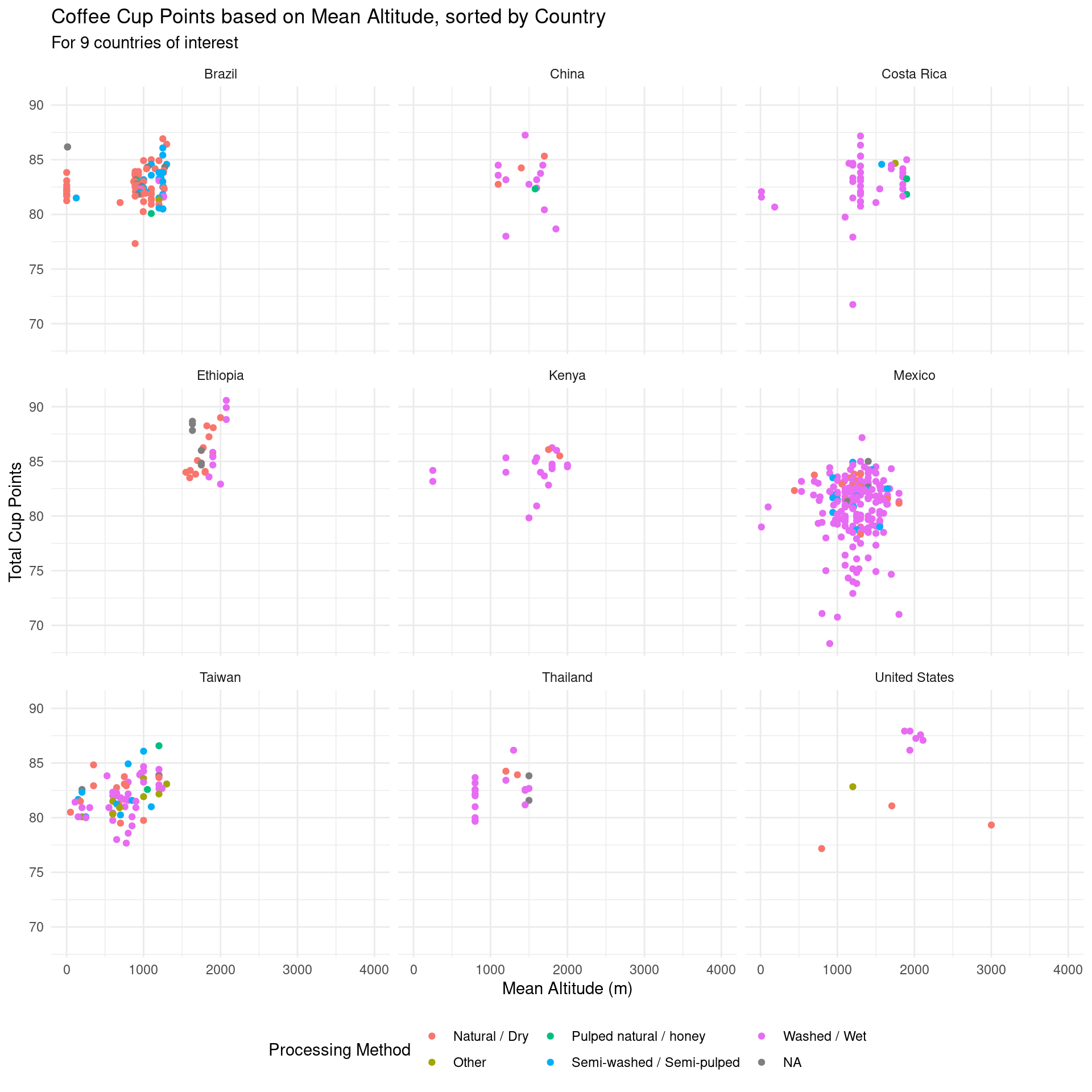
# A tibble: 9 × 2
  country_of_origin mean_cup_points
  <chr>                       <dbl>
1 Ethiopia                     86.1
2 United States                84.4
3 Kenya                        84.2
4 China                        82.9
5 Costa Rica                   82.8
6 Brazil                       82.7
7 Thailand                     82.4
8 Taiwan                       81.9
9 Mexico                       80.9
When looking at processing method, it was interesting to see how different countries specialized in different methods. Coffee ratings seem to differ more based on the country they are from compared to the altitude of which they are grown, which may imply that processing method has a larger impact on the ratings than altitude. After some research, we found that processing method effects flavor and aroma of coffee. To better understand this difference, we looked at the effect of processing method on these aspects of coffee taste.
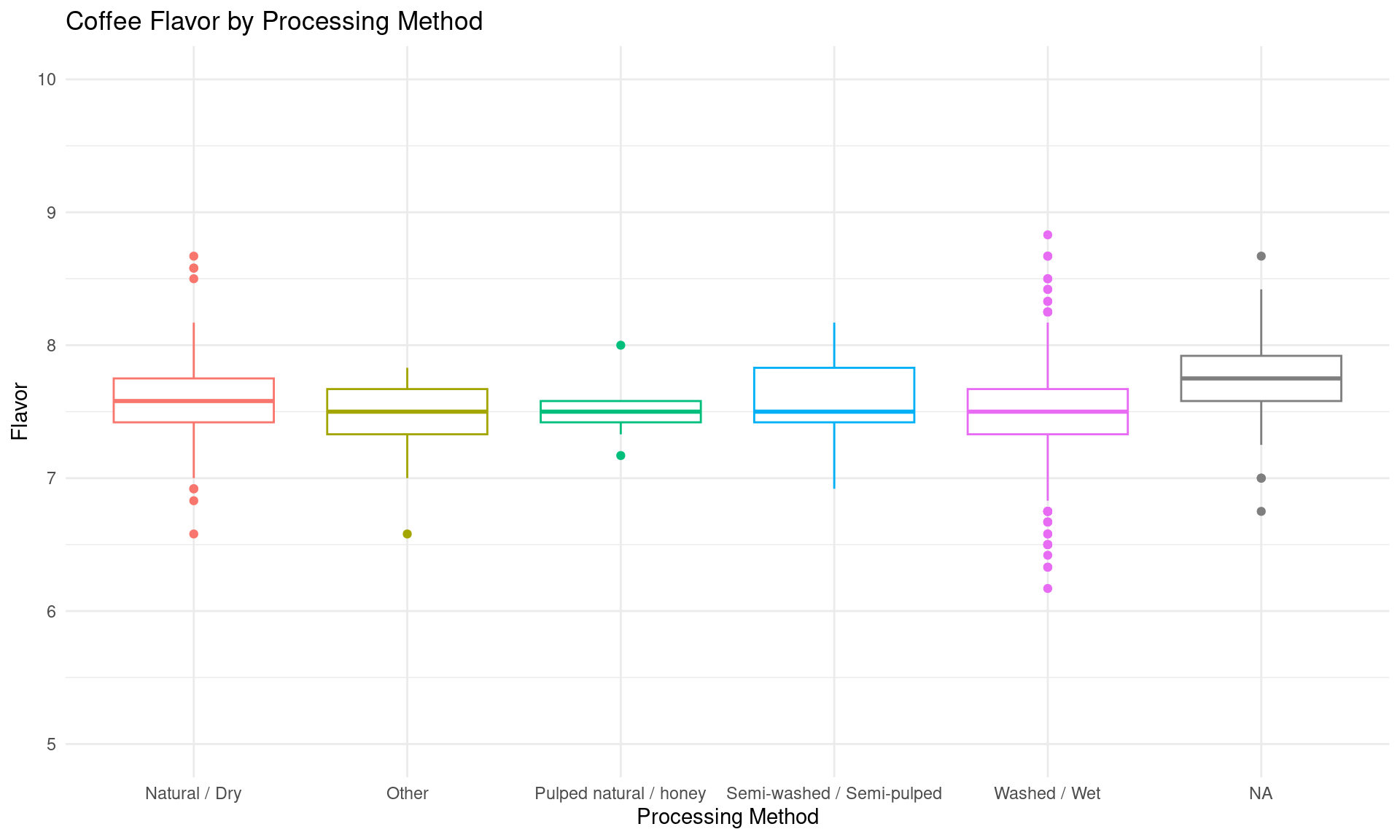
coffee_ratings_clean |>ggplot(mapping =aes(x = processing_method, y = flavor, color = processing_method)) +geom_boxplot() +labs(x ="Processing Method", y ="Flavor", title ="Coffee Flavor by Processing Method" ) +scale_y_continuous(limits =c(5, 10)) +guides(color =FALSE) +theme_minimal()
Warning: The `<scale>` argument of `guides()` cannot be `FALSE`. Use "none" instead as
of ggplot2 3.3.4.
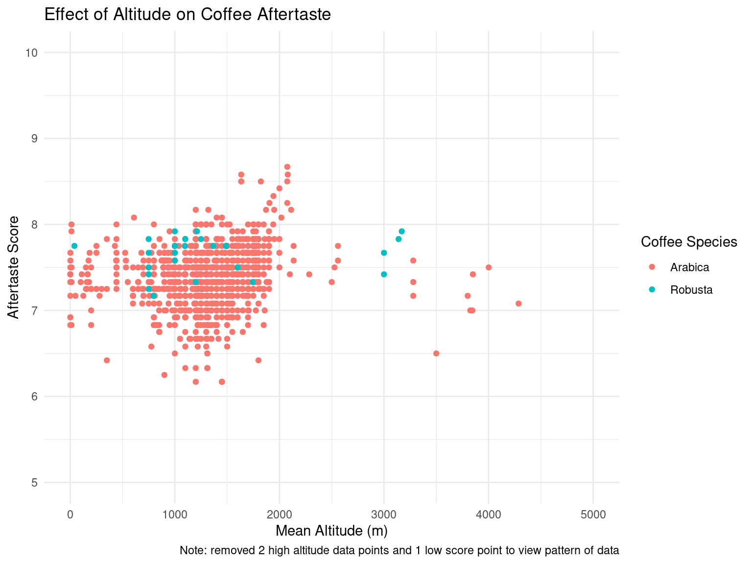
After the exploratory data analysis, it is difficult to see any particular impact that altitude or processing method has on taste scores for coffee. However, there is an interesting range of altitudes where total cup points and taste scores tend to increase slightly, up until a range of “ideal altitudes”. We could further investigate this trend as our project moves forward. There is also a slight difference in aroma and flavor scores for different processing methods, although it is difficult to tell if this arises by chance. For example, the Washed/Wet processing method tends to produce less consistent results in aroma and flavor while the Pulped natural/honey method gives very consistent results. However, this could easily be caused by the frequency of which each processing method is used. This would also be interesting to look into in the future.
Questions for reviewers
List specific questions for your peer reviewers and project mentor to answer in giving you feedback on this phase.
Is the scope of our research question too wide or too narrow?
Should we switch our research question after not finding an obvious relationship between the mean altitude and coffee taste scores?