UFO Sighting Patterns Across Education, Politics, and Time

Author

Red-Koala
Asad Nabi, Fiona Yang, Angela Yuan

── Attaching core tidyverse packages ──────────────────────── tidyverse 2.0.0 ──
✔ dplyr     1.1.4     ✔ readr     2.1.5
✔ forcats   1.0.0     ✔ stringr   1.5.1
✔ ggplot2   3.4.4     ✔ tibble    3.2.1
✔ lubridate 1.9.3     ✔ tidyr     1.3.0
✔ purrr     1.0.2     
── Conflicts ────────────────────────────────────────── tidyverse_conflicts() ──
✖ dplyr::filter() masks stats::filter()
✖ dplyr::lag()    masks stats::lag()
ℹ Use the conflicted package (<http://conflicted.r-lib.org/>) to force all conflicts to become errors

Attaching package: 'scales'


The following object is masked from 'package:purrr':

    discard


The following object is masked from 'package:readr':

    col_factor



Attaching package: 'janitor'


The following objects are masked from 'package:stats':

    chisq.test, fisher.test



Attaching package: 'gridExtra'


The following object is masked from 'package:dplyr':

    combine

Rows: 96429 Columns: 12
── Column specification ────────────────────────────────────────────────────────
Delimiter: ","
chr  (7): city, state, country_code, shape, reported_duration, summary, day_...
dbl  (1): duration_seconds
lgl  (1): has_images
dttm (2): reported_date_time, reported_date_time_utc
date (1): posted_date

ℹ Use `spec()` to retrieve the full column specification for this data.
ℹ Specify the column types or set `show_col_types = FALSE` to quiet this message.
Rows: 14417 Columns: 10
── Column specification ────────────────────────────────────────────────────────
Delimiter: ","
chr (6): city, alternate_city_names, state, country, country_code, timezone
dbl (4): latitude, longitude, population, elevation_m

ℹ Use `spec()` to retrieve the full column specification for this data.
ℹ Specify the column types or set `show_col_types = FALSE` to quiet this message.
Rows: 26409 Columns: 12
── Column specification ────────────────────────────────────────────────────────
Delimiter: ","
dbl  (2): rounded_lat, rounded_long
date (1): rounded_date
time (9): astronomical_twilight_begin, nautical_twilight_begin, civil_twilig...

ℹ Use `spec()` to retrieve the full column specification for this data.
ℹ Specify the column types or set `show_col_types = FALSE` to quiet this message.

Introduction

TidyTuesday’s UFO sightings dataset:

The dataset is a culmination of 3 CSV files

ufo_sightings.csv
- This csv file gives information about when, where, how, and important information pertinent to the sighting itself
places.csv
- Gives additional information about the place itself
day_parts_map.csv
- Gives information about the sunrise, sunset, and astronomy information about the day in particular

Are the prevalence of UFO reports related to states with lower literacy rates or certain political leanings?

Introduction

(1-2 paragraphs) Introduction to the question and what parts of the dataset are necessary to answer the question. Also discuss why you’re interested in this question.

In this case, we are interested in seeing where UFO reports generally come from and if it’s related to places with lower literacy rates or certain political affiliations (Conservative and Democratic). To answer this question, we will import two datasets, one with states and their respective low literacy rates (percentage of illiterate individuals) and the other with states and their respective political affiliation (via governor party). In the UFO datasets, we need the states and frequency at which a UFO reports happen in a state

Approach

In the UFO datasets, we need the states and will use data wrangling to find the frequency at which a UFO reports happen in a state. Furthermore, from the other datsets, we will grab the low literacy rates and the states with respective political affiliation. We will join these datasets together by the state and use these variables to count the frequency at which a UFO reports happen in a state. Firstly, using this we will create a scatter plot with lower-literacy rates (X axis) vs number of UFO sightings (Y axis). We will also have a line of best fit to further see the trend. A scatter chart with a line of best fit is the optimal way to show relationship between two continuous variables. To coincide with this, we will have a barchart with UFO sightings given that it was from a conservative-leaning state and sightings given that it was from a liberal-leaning state and compare the results. We have a discrete and continuous variable and as such, the bar chart is the best to showcase the relation.

Analysis

UFO sighting relative to literacy rates

#data from https://worldpopulationreview.com/state-rankings/us-literacy-rates-by-state
literacy_rates <- read.csv("data/us-literacy-rates-by-state-2024.csv") |>
  clean_names() |>
  rename("pct_of_low_literacy" = literacy_rates_percof_population_with_low_literacy,
         "reading_level" = literacy_rates_percof4th_graders_below_basic_reading_level) |>
  select(state, pct_of_low_literacy) |>
  mutate(
    state = state.abb[match(state,state.name)]
  ) 

ufo_sightings_us <- ufo_sightings |>
  filter(country_code == "US")
  
ufo_state_literacy_rates <- left_join(ufo_sightings_us, literacy_rates, by="state")

ufo_state_literacy_rates |>
  drop_na() |>
  select(state, pct_of_low_literacy) |>
  mutate(
    number_of_ufo_sightings = as.numeric(ave(state, state, FUN = length))
  ) |>
  arrange(state) |> unique() |> 
  ggplot(aes(x=pct_of_low_literacy, y=number_of_ufo_sightings)) +
  geom_text(label=fontawesome('fa-rocket'), 
            family='fontawesome-webfont', size=8, alpha=0.7, color="darkred") +
  geom_smooth(method = "lm", se = FALSE, color="red") +
  ylim(-100,6000) +
  theme_minimal() +
  scale_x_continuous(labels = label_percent(scale=1)) +
  labs(
    x = "Percentage of population with low literacy",
    y = "Number of UFO sightings",
    title = "UFO sightings and literacy rates"
  )

`geom_smooth()` using formula = 'y ~ x'

Warning: Removed 1 rows containing non-finite values (`stat_smooth()`).

Warning: Removed 1 rows containing missing values (`geom_text()`).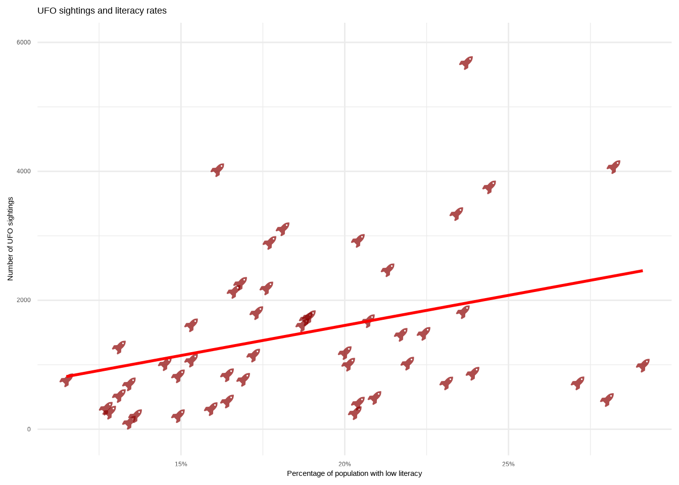

UFO sighting relative to political leaning

politic <- read_csv("data/political_states.csv") |>
  clean_names() |>
  rename("state" = location) |>
  mutate(
    state = state.abb[match(state,state.name)]
  ) |>
  drop_na() |>
  select(state, governor_political_affiliation)

Rows: 52 Columns: 6
── Column specification ────────────────────────────────────────────────────────
Delimiter: ","
chr (6): Location, Governor Political Affiliation, State Senate Majority Pol...

ℹ Use `spec()` to retrieve the full column specification for this data.
ℹ Specify the column types or set `show_col_types = FALSE` to quiet this message.

ufo_politic <- left_join(ufo_state_literacy_rates, politic, by="state")

ufo_politic |>
  select(state, governor_political_affiliation) |>
  mutate(
    number_of_ufo_sightings = as.numeric(ave(state, state, FUN = length)),
  ) |> rename(political_leaning = governor_political_affiliation) |>
  drop_na() |> arrange(state) |> unique() |>
  ggplot(aes(x=political_leaning, y=number_of_ufo_sightings, fill = political_leaning)) +
  geom_bar(stat="identity") + 
  scale_fill_manual(values=c("blue", "red")) +
  theme_minimal() +
    labs(
    x = "Political Leaning",
    y = "Number of UFO sightings",
    title = "UFO sightings and literacy rates",
  ) + theme(legend.position = "none")

Discussion

(1-3 paragraphs) In the Discussion section, interpret the results of your analysis. Identify any trends revealed (or not revealed) by the plots. Speculate about why the data looks the way it does.

In the first graph, with the percentage with low literacy being in the x axis, and number of UFO sightings in the y axis, we can see increase in UFO sightings when there is a larger porportion in the population with a lower literacy rate. In other words, as the lower-literacy rate (percentage of individuals who are illiterate) increases of a state/region, the number of UFO sightings increase.

In the second graph, we see that Democrat represented states have an overall more UFO sightings then Republican represented states.

We recognize overall there could be confounding factors such as population density or age which may be unaccounted for, but we are claiming solely a correlation.

Seasonal Frequency of UFO Sighting over the years.

Introduction

Question: During what part of year is UFO sighting more frequent and how does these trends change over the years? By categorizing these sightings into seasons—Spring, Summer, Autumn, and Winter—we can explore whether certain times of the year are more prone to such phenomena. `posted_date, which are the posted date of UFO sightings, will be used to answer the question.

Approach

To analyze the temporal distribution of UFO sightings, two distinct types of plots will be employed: a bar plot and a line plot. The bar plot will be utilized to represent the frequency of sightings across different seasons, offering a clear visual comparison between Spring, Summer, Autumn, and Winter. This choice is motivated by the bar plot’s effectiveness in showcasing categorical data and making it easy to compare the number of sightings across the four predefined seasons. Color mapping will be used within this plot to differentiate between the seasons, providing an immediate visual cue to the viewer.

On the other hand, a line plot will be created to illustrate how the frequency of UFO sightings has evolved over the years. This type of plot is chosen for its ability to display trends over time, allowing for an analysis of whether sightings have become more or less frequent and if there are any discernible patterns correlating with specific periods or events.

Analysis

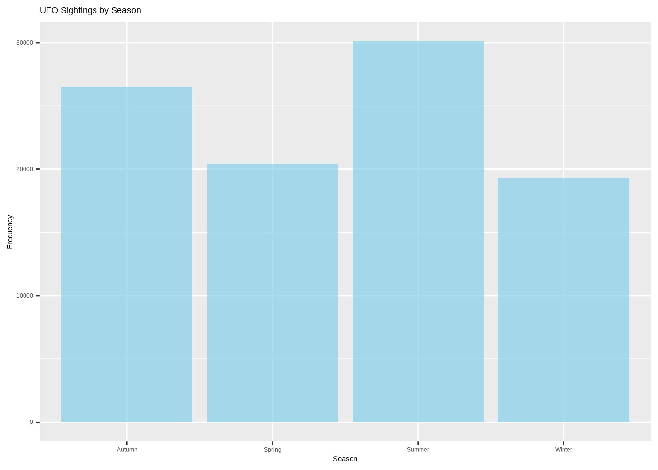
UFO Sighting Frequency by Season

ufo_sightings$month <- lubridate::month(ufo_sightings$reported_date_time)

ufo_sightings <-
ufo_sightings |>
  mutate(season = case_when(
      month %in% 3:5 ~ "Spring",
      month %in% 6:8 ~ "Summer",
      month %in% 9:11 ~ "Autumn",
      TRUE ~ "Winter"
  )) 

ufo_sightings |>

ggplot(aes(x = season)) +
  geom_bar(fill = "skyblue", alpha = 0.7) +
  labs(
    x = "Season",
    y = "Frequency",
    title = "UFO Sightings by Season"

)

UFO Sighting Season Trend Over Time

ufo_sightings$posted_date <- as.Date(ufo_sightings$posted_date)

ufo_sightings$year <- year(ufo_sightings$posted_date)

sightings_summary <- ufo_sightings %>%
  group_by(season, year) %>%
  summarise(Frequency = n())

`summarise()` has grouped output by 'season'. You can override using the
`.groups` argument.

ggplot(sightings_summary, aes(x = year, y = Frequency, color = season, group = season)) +
  geom_line() +
  geom_point() +
  theme_minimal() +
  labs(title = "Frequency of Sightings Over Time by Season",
       x = "Year",
       y = "Frequency of Sightings") +
  scale_color_manual(
    values = c("Spring" = "pink", "Summer" = "lightgreen", 
               "Autumn" = "orange", "Winter" = "lightblue"))

Discussion

(1-3 paragraphs) In the Discussion section, interpret the results of your analysis. Identify any trends revealed (or not revealed) by the plots. Speculate about why the data looks the way it does.

According to the results, for the first graph, UFO Sighting Frequency by Season, we discovered that UFO sightings tend to be more frequent in summer and autumn than spring and winter. One possible cause is the correlation of summer with increased outdoor activities, increasing the chance of spotting an ufo. For the second graph, it reconfirms the summer as the prime time to spot and report an ufo. The trend for all seasons increased up to the peak in 2014, then reached a drastic decline until around 2018. This is possibly related to the news that in 2015, Californians called law enforcement regarding an “UFO”, a bright light cutting through the sky, which turnd out to be a test missile of the US Navy. This may have dampened the enthusiasm of the reporting crowd.

National UFO Reporting Center

Link to an article with theories of why ufo sightings spike in the summer: https://www.businessinsider.com/why-ufo-sightings-peak-in-the-summer-2016-2

Presentation

Our presentation can be found here.

Data

Include a citation for your data here. See http://libraryguides.vu.edu.au/c.php?g=386501&p=4347840 for guidance on proper citation for datasets. If you got your data off the web, make sure to note the retrieval date.

UFO Sighting Dataset: https://github.com/rfordatascience/tidytuesday/blob/master/data/2023/2023-06-20/readme.md

literacy rates dataset - https://worldpopulationreview.com/state-rankings/us-literacy-rates-by-state (02/28/2024)

state political parties dataset - https://www.kff.org/other/state-indicator/state-political-parties/?currentTimeframe=0&sortModel=%7B%22colId%22:%22Location%22,%22sort%22:%22asc%22%7D (02/28/2024)

References

UFO Sighting Dataset: https://github.com/rfordatascience/tidytuesday/blob/master/data/2023/2023-06-20/readme.md

literacy rates dataset - https://worldpopulationreview.com/state-rankings/us-literacy-rates-by-state

state political parties dataset - https://www.kff.org/other/state-indicator/state-political-parties/?currentTimeframe=0&sortModel=%7B%22colId%22:%22Location%22,%22sort%22:%22asc%22%7D