── Attaching core tidyverse packages ──────────────────────── tidyverse 2.0.0 ──
✔ dplyr     1.1.4     ✔ readr     2.1.5
✔ forcats   1.0.0     ✔ stringr   1.5.1
✔ ggplot2   3.5.1     ✔ tibble    3.2.1
✔ lubridate 1.9.4     ✔ tidyr     1.3.1
✔ purrr     1.0.4
── Conflicts ────────────────────────────────────────── tidyverse_conflicts() ──
✖ dplyr::filter() masks stats::filter()
✖ dplyr::lag()    masks stats::lag()
ℹ Use the conflicted package (<http://conflicted.r-lib.org/>) to force all conflicts to become errors

Attaching package: 'scales'


The following object is masked from 'package:purrr':

    discard


The following object is masked from 'package:readr':

    col_factor


Attaching package: 'janitor'


The following objects are masked from 'package:stats':

    chisq.test, fisher.test


Loading required package: viridisLite


Attaching package: 'viridis'


The following object is masked from 'package:scales':

viridis_palAnalyzing Global Entity Carbon Emissions
To-Do
- Glossary for uncommon language and categorical variables
Set-up
theme_proj1 <- function() {
  theme_light() +
    theme(
      plot.title.position = "plot",
      legend.position = "top",
      plot.title = element_text(
        hjust = 0.5,
        face = "bold"
      ),
      plot.subtitle = element_text(hjust = 0.5),
      legend.text = element_text(size = 6),
      legend.key.size = unit(3, "mm"),
      legend.background = element_rect(color = "grey"),
      panel.grid.major.x = element_line(color = "grey"),
      panel.grid.minor.x = element_line(color = "grey"),
      panel.grid.major.y = element_line(color = "grey"),
      panel.grid.minor.y = element_line(color = "grey"),
      axis.text.x = element_text(
        hjust = 1
      ),
      strip.text = element_text(
        color = "white",
        face = "bold"
      ),
      strip.background = element_rect(
        fill = "black",
        linewidth = 0.5
      ),
      axis.ticks.length = unit(
        1.5,
        "mm"
      ),
      axis.line = element_line(
        color = "black"
      ),
      axis.title = element_text(
        face = "bold"
      )
    )
}

theme_set(theme_proj1())
Data cleaning
em <- emissions |>
  mutate(
    year = ym(paste0(year, "-01")),
    tot_opem_mt = as.numeric(total_operational_emissions_mt_co2e),
    tot_em_mt = as.numeric(total_emissions_mt_co2e),
    tot_prodem_mt = as.numeric(product_emissions_mt_co2)
  )
Warning: There were 4 warnings in `mutate()`.
The first warning was:
ℹ In argument: `year = ym(paste0(year, "-01"))`.
Caused by warning:
! 3 failed to parse.
ℹ Run `dplyr::last_dplyr_warnings()` to see the 3 remaining warnings.Introduction
(1-2 paragraphs) Brief introduction to the dataset. You may repeat some of the information about the dataset provided in the introduction to the dataset on the TidyTuesday repository, paraphrasing on your own terms. Imagine that your project is a standalone document and the grader has no prior knowledge of the dataset.
Why we chose this data set:
Our generation, Generation Z, has grown up with the climate crisis looming over our heads. When our group examined the available data sets from TidyTuesday, there were more than a handful of perfectly viable choices for our project. In the end our team chose this data set because of its relevance to our futures and the possible stories that could be revealed through the data. On a more technical scale, the “parent_type” column is of particular interest to our team because of the possible socioeconomic implications that may arise from categorical patterns.
Dataset History/Provenance:
We chose to explore the Carbon Majors dataset, which tracks emissions from major fossil fuel and cement producers since 1854. The dataset was originally created by Richard Heede of the Climate Accountability Institute in 2013. In April 2024, InfluenceMap took over the maintenance and annual updates of the dataset, releasing it on carbonmajors.org. The dataset covers 122 of the world’s largest oil, gas, coal, and cement producers, including investor-owned companies, state-owned entities, and nation-states. It provides a comprehensive view of these entities’ contributions to greenhouse gas emissions, accounting for about 72% of global fossil fuel and cement emissions since the Industrial Revolution. The data is available in three granularity levels (low, medium, and high), offering different levels of detail on emissions and production.
Description:
CarbonsMajors emission data (high granularity) data set provides information on historical carbon emissions from 122 of the world’s largest oil, gas, coal, and cement producers spanning back to 1854. The data set provides information across various parent entities, including investor-owned companies, state-owned entities, and nation states. It also tracks emissions from different fossil fuel commodities, along with production volumes and the unit of production.
glimpse(emissions)Rows: 31,597
Columns: 16
$ year <chr> "1962", "1963", "1964", "1965", "1…
$ parent_entity <chr> "Abu Dhabi National Oil Company", …
$ parent_type <chr> "State-owned Entity", "State-owned…
$ reporting_entity <chr> "Abu Dhabi", "Abu Dhabi", "Abu Dha…
$ commodity <chr> "Oil & NGL", "Oil & NGL", "Oil & N…
$ production_value <chr> "0.9125", "1.825", "7.3", "10.95",…
$ production_unit <chr> "Million bbl/yr", "Million bbl/yr"…
$ product_emissions_mt_co2 <chr> "0.3389277", "0.677855399", "2.711…
$ flaring_emissions_mt_co2 <chr> "0.005404077", "0.010808155", "0.0…
$ venting_emissions_mt_co2 <chr> "0.001298972", "0.002597944", "0.0…
$ own_fuel_use_emissions_mt_co2 <chr> "0.00E+00", "0.00E+00", "0.00E+00"…
$ fugitive_methane_emissions_mt_co2e <chr> "0.018254082", "0.036508164", "0.1…
$ fugitive_methane_emissions_mt_ch4 <chr> "0.000651931", "0.001303863", "0.0…
$ total_operational_emissions_mt_co2e <chr> "0.024957131", "0.049914263", "0.1…
$ total_emissions_mt_co2e <chr> "0.363884831", "0.727769662", "2.9…
$ source <chr> "Abu Dhabi National Oil Company An…skim(emissions)| Name | emissions |
| Number of rows | 31597 |
| Number of columns | 16 |
| _______________________ | |
| Column type frequency: | |
| character | 16 |
| ________________________ | |
| Group variables | None |
Variable type: character
| skim_variable | n_missing | complete_rate | min | max | empty | n_unique | whitespace |
|---|---|---|---|---|---|---|---|
| year | 0 | 1 | 4 | 48 | 0 | 172 | 0 |
| parent_entity | 0 | 1 | 0 | 39 | 2 | 125 | 0 |
| parent_type | 0 | 1 | 0 | 22 | 2 | 5 | 0 |
| reporting_entity | 0 | 1 | 0 | 42 | 2 | 308 | 0 |
| commodity | 0 | 1 | 0 | 19 | 2 | 11 | 0 |
| production_value | 0 | 1 | 0 | 16 | 2 | 13835 | 0 |
| production_unit | 0 | 1 | 0 | 18 | 2 | 6 | 0 |
| product_emissions_mt_co2 | 0 | 1 | 0 | 23 | 2 | 14523 | 0 |
| flaring_emissions_mt_co2 | 0 | 1 | 0 | 23 | 2 | 9141 | 0 |
| venting_emissions_mt_co2 | 0 | 1 | 0 | 23 | 2 | 9141 | 0 |
| own_fuel_use_emissions_mt_co2 | 0 | 1 | 0 | 28 | 2 | 4372 | 0 |
| fugitive_methane_emissions_mt_co2e | 0 | 1 | 0 | 33 | 2 | 14217 | 0 |
| fugitive_methane_emissions_mt_ch4 | 0 | 1 | 0 | 32 | 2 | 14215 | 0 |
| total_operational_emissions_mt_co2e | 0 | 1 | 0 | 34 | 2 | 14217 | 0 |
| total_emissions_mt_co2e | 0 | 1 | 0 | 22 | 2 | 14523 | 0 |
| source | 0 | 1 | 0 | 372 | 2 | 2241 | 0 |
dim_text <- paste("The dataset has", nrow(emissions), "rows and", ncol(emissions), "columns.")
print(dim_text)
[1] "The dataset has 31597 rows and 16 columns."Defining key terms.
-
- “…four direct operational emissions sources. Note these are only partial scope 1 emissions, only emissions that are production-linked. An entity’s total scope 1 emissions may be higher…”
-
- “…emissions from the combustion of marketed products. Note these are partial scope 3 emissions categorized as Scope 3: Category 11 ‘use of sold products’, which has been modified to quantify emissions from each entity’s net production as opposed to sold products. An entity’s total scope 3 emissions may be higher…”
-
- “…companies often partially owned by institutional or individual shareholders. These are considered state owned if more than fifty percent of shares are controlled by the state…”
-
- “…producers used primarily in the coal sector and are included only when investor-owned or state-owned companies haven’t been established or played a minor role in the relevant country. Examples include North Korea and former Soviet states…”
-
- …companies both publicly listed and privately held producers…”
Examining overarching emission patterns across entity types.
Question 1: Do different entity types have different emission patterns over time, and are pattern changes related to enacted major climate conscious legislation?
Introduction
(1-2 paragraphs) Introduction to the question and what parts of the dataset are necessary to answer the question. Also discuss why you’re interested in this question.
Question 1 dives deeper into the climate crisis by probing at the relationship between entity type of fossil fuel producers and the emissions they create. Furthermore, our team wanted to highlight years where regional or international climate conscious legislation was passed. Adding this additional context enables our team to identify whether or not the legislation impacted fossil fuel emissions in the long run. Additionally, by grouping by entity type we can analyze the reactions of each entity type.
Chosen Climate Conscious Legislation
Montreal Protocol (Effective 1989)
U.S. Clean Air Act Amendments (1990)
Kyoto Protocol (Implemented 2005)
European Union Emissions Trading System (EU ETS) (2005)
UK Climate Change Act (2008)
UK Climate Change Act (2008)
Paris Climate Agreement (Implemented 2016)
Approach
(1-2 paragraphs) Describe what types of plots you are going to make to address your question. For each plot, provide a clear explanation as to why this plot (e.g. boxplot, barplot, histogram, etc.) is best for providing the information you are asking about. The two plots should be of different types, and at least one of the two plots needs to use either color mapping or facets.
Variables created by the team
avg_em
- The average annual emissions of all entities in a given entity type
p_year_em
- An entity type’s proportion of a year’s TOTAL emissions
In order to further tailor our data to Question 1, we decided to use data between 1975 and 2022 because most regional/international climate conscious legislation was not passed until the latter half of the twentieth century. After filtering our data we created new variables to summarize the patterns we wanted to examine:
When it came to visualizing our data, we initially planned on using only bar plots and column graphs. However, we realized that a ridgeline plot would provide us a more detailed and efficient look at patterns over time. In addition to the ridgeline polygons, our team added vertical lines to our first visualization that indicate when our chosen legislation was enacted. However, due to the nature of ggridgelines there is no way to understand the numeric value at a given point, so we decided to add labels and points that explicitly state each entity type’s average emissions for years where our chosen climate conscious legislation was passed.
After we created the first visualization we saw that the entity type “Nation State” had large emission rates, and decided to try and account for this. Rather than taking just the average emissions, we wanted to see how the composition of emissions changed each year across entity types. In other words, what percentage of a year’s emissions were made up by each entity type? Here is where our team returned to our initial inclination to bar plots. Upon first visualization we really liked a stacked view, however this made it difficult to understand the patterns for each individual entity type, so we decided that a dodged barplot would be ideal.
Analysis
q1data <- em |>
  select(
    parent_type,
    year,
    tot_em_mt
  ) |>
  group_by(
    parent_type,
    year
  ) |>
  summarise(
    avg_em = mean(tot_em_mt)
  ) |>
  filter(
    !is.na(avg_em)
  ) |>
  mutate(
    parent_type = factor(
      parent_type,
      levels = c(
        "Investor-owned Company",
        "State-owned Entity",
        "Nation State"
      )
    )
  ) |>
  distinct()
`summarise()` has grouped output by 'parent_type'. You can override using the
`.groups` argument.years <- c(
ym("2022-01"),
ym("1989-01"),
ym("1990-01"),
ym("2005-01"),
ym("2005-01"),
ym("2016-01"),
ym("2008-01")
)
labs <- q1data |>
filter(
year %in% years
)
q1data2 <- em |>
filter(
!is.na(tot_em_mt)
) |>
select(
parent_type,
year,
tot_em_mt
) |>
group_by(
year
) |>
mutate(
tot_year_em = sum(tot_em_mt)
) |>
group_by(
parent_type,
year
) |>
reframe(
ent_year_em = sum(tot_em_mt),
parent_type,
year,
tot_year_em
) |>
reframe(
p_year_em = ent_year_em / tot_year_em,
year,
parent_type
) |>
mutate(
entity_type = factor(
parent_type,
levels = c(
"Investor-owned Company",
"State-owned Entity",
"Nation State"
)
)
) |>
distinct()
labs2 <- q1data2 |>
filter(
year %in% years
)q1vis <-
ggplot() +
geom_ridgeline(
data = q1data,
aes(
x = year,
y = parent_type,
height = avg_em,
fill = parent_type,
color = parent_type
),
alpha = 0.7
) +
scale_fill_viridis_d(
name = "Entity Type",
begin = 0.4,
end = 0.95
) +
scale_color_viridis_d(
name = "Entity Type",
begin = 0.4,
end = 0.95
) +
new_scale_color() +
geom_vline(
data = events,
aes(
xintercept = year,
color = factor(year)
),
linewidth = 0.8
) +
geom_point(
data = labs,
aes(
x = year,
y = avg_em,
color = factor(year),
shape = parent_type
),
size = 2,
show.legend = FALSE
) +
scale_color_viridis_d(
name = "Climate Forward
Legislation",
option = "magma",
begin = 0.2,
end = 0.7,
labels = c(
"1989: Montreal Protocol",
"1990: U.S. Clean Air Act Amendments",
"2005: Kyoto Protocol and
EU Emissions Trading System",
"2008: UK Climate Change Act",
"2016: Paris Climate Agreement",
""
)
) +
new_scale_color() +
geom_label_repel(
data = labs,
aes(
x = year,
y = avg_em,
label = paste0(round(avg_em), " mt CO2"),
fill = parent_type
),
size = 2,
fontface = "bold",
min.segment.length = 0.1,
label.r = 0.25,
show.legend = FALSE
) +
scale_fill_viridis_d(
name = "Entity Type",
begin = 0.6,
end = 0.95
) +
scale_color_viridis_d(
name = "Entity Type",
begin = 0.4,
end = 0.95
) +
scale_x_date(
name = "Year",
limits = c(ym("1975-01"), ym("2025-01")),
breaks = "10 years",
date_labels = "%Y"
) +
scale_y_discrete(
name = "Annual Emissions (Mt CO2)"
) +
theme(
legend.position = "right",
axis.text.y = element_blank(),
axis.text.x = element_text(
hjust = 0.5
)
) +
labs(
title = "Average Annual Emissions (Mt CO2) Across Entity Types (1972-2022)"
)Scale for fill is already present.
Adding another scale for fill, which will replace the existing scale.q1vis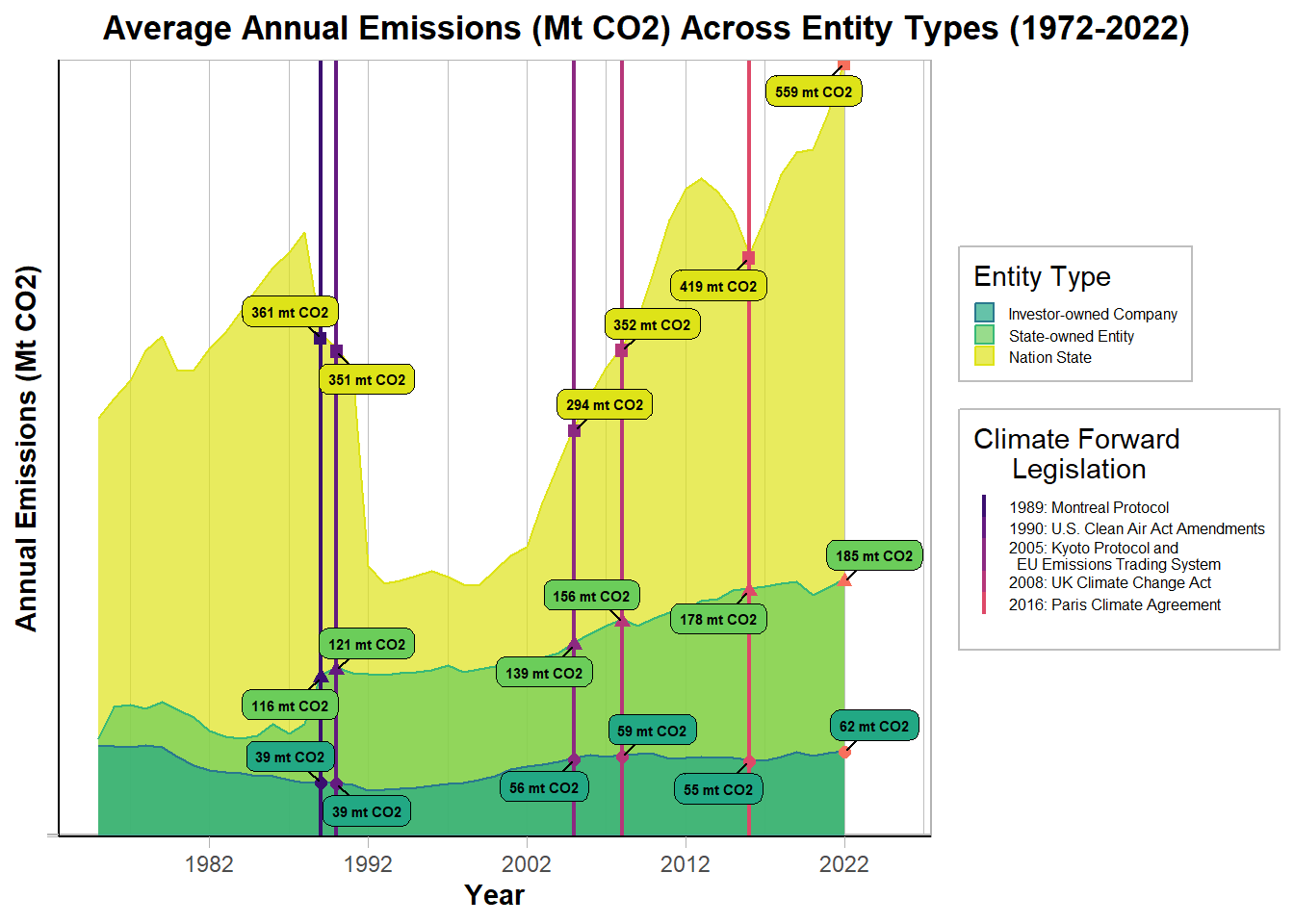
q1vis2 <- ggplot() +
  geom_col(
    data = q1data2,
    aes(
      x = year,
      y = p_year_em,
      fill = factor(parent_type)
    ),
    show.legend = FALSE
  ) +
  facet_wrap(~parent_type, ncol = 1) +
  scale_fill_viridis_d(
    begin = 0.4,
    end = 0.95
  ) +
  scale_color_viridis_d(
    begin = 0.4,
    end = 0.95
  ) +
  new_scale_color() +
  geom_vline(
    data = events,
    aes(
      xintercept = year,
      color = factor(year)
    ),
    linewidth = 0.8
  ) +
  geom_point(
    data = labs2,
    aes(
      x = year,
      y = p_year_em,
      color = factor(year),
      shape = parent_type
    ),
    size = 2,
    show.legend = FALSE
  ) +
  scale_color_viridis_d(
    name = "Climate Forward
     Legislation",
    option = "magma",
    begin = 0.2,
    end = 0.7,
    labels = c(
      "1989: Montreal Protocol",
      "1990: U.S. Clean Air Act Amendments",
      "2005: Kyoto Protocol and
  EU Emissions Trading System",
      "2008: UK Climate Change Act",
      "2016: Paris Climate Agreement",
      ""
    )
  ) +
  new_scale_color() +
  geom_label_repel(
    data = labs2,
    aes(
      x = year,
      y = p_year_em,
      label = paste0(round(p_year_em * 100, 1), "%"),
      fill = parent_type
    ),
    size = 2,
    fontface = "bold",
    min.segment.length = 0.1,
    label.r = 0.25,
    show.legend = FALSE
  ) +
  scale_fill_viridis_d(
    name = "Entity Type",
    begin = 0.6,
    end = 0.95
  ) +
  scale_color_viridis_d(
    name = "Entity Type",
    begin = 0.4,
    end = 0.95
  ) +
  scale_x_date(
    name = "Year",
    limits = c(ym("1975-01"), ym("2025-01")),
    breaks = "5 years",
    date_labels = "%Y"
  ) +
  scale_y_continuous(
    name = "Percentage of Annual CO2 Emissions",
    labels = percent,
    limits = c(0, 0.60)
  ) +
  theme(
    legend.position = "right",
    panel.grid.minor.y = element_blank(),
    panel.grid.minor.x = element_blank(),
    axis.text.x = element_text(
      hjust = 0.5
    )
  ) +
  labs(
    title = "Percentage of Total Annual Emissions
    (Mt CO2) Across Entity Types (1975-2022)"
  )
Scale for fill is already present.
Adding another scale for fill, which will replace the existing scale.print(q1vis2)Warning: Removed 246 rows containing missing values or values outside the scale range
(`geom_col()`).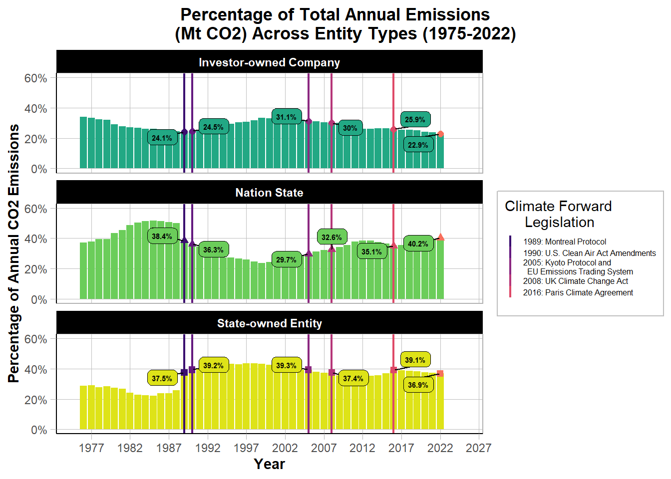
Discussion
The analysis of CO2 emissions across different entity types reveals distinct patterns over time, particularly in relation to major climate policy interventions. Investor-owned companies have maintained relatively stable contributions to global emissions, with a slight decline in recent years. Despite policy interventions such as the Kyoto Protocol (2005) and the Paris Climate Agreement (2016), their emissions remain significant, suggesting that market-driven companies may respond to regulation but do not dramatically alter emissions output without stronger enforcement or economic incentives.
State-owned entities have shown a more consistent share of emissions, fluctuating around the 35–40% range. While there are observable declines following certain policy enactments, these reductions are not sustained. The relatively stable trend suggests that state-owned entities, often tied to national energy policies, may not be as responsive to global climate initiatives as investor-owned firms. Nation-states exhibit the most variation in emissions contributions, with notable peaks and declines. While their share of total emissions has fluctuated, recent data shows an increasing trend, reaching over 40% in 2022. This rise suggests that some countries, despite global climate commitments, continue to increase fossil fuel dependence. The limited and inconsistent impact of policy interventions highlights the challenges of enforcing international agreements at the state level.
Overall, while climate policies have led to some reductions or temporary shifts, emissions remain persistently high across all entity types. This shows the need for stronger enforcement mechanisms, financial incentives, and technological innovations to achieve meaningful, long-term reductions in carbon output.
Examining Scope 1 and Scope 3 emissions across entity and commodity types.
Question 2: How do Scope 1 and Scope 3 emissions change over time across commodity and entity types?
Introduction
(1-2 paragraphs) Introduction to the question and what parts of the dataset are necessary to answer the question. Also discuss why you’re interested in this question.
Greenhouse gas emissions from fossil fuel production play a crucial role in the global climate crisis. Understanding the differences between Scope 1 (direct operational emissions) and Scope 3 (product-related emissions) across different commodity types—Coal, Natural Gas, and Oil & NGL, is essential for evaluating how non-investor-owned entities contribute to total carbon output. These entities, which include state-owned enterprises and nation-states, operate under distinct economic and regulatory conditions compared to investor-owned companies. Their emissions patterns may reflect governmental priorities, energy policies, or national economic dependencies on fossil fuel exports. Investigating these patterns can provide insight into whether emissions mitigation efforts should focus more on operational reductions (Scope 1) or end-user impacts (Scope 3) and help focus our efforts in lowering CO2 emissions into the right places.
This analysis leverages the Carbon Majors data set, specifically focusing on the “parent_type,” “commodity,” “total_operational_emissions_mt_co2e,” and “product_emissions_mt_co2” variables to assess how emissions are distributed across different commodity types. We extracted annual emission data from non-investor-owned entities and processed it to determine the average operational and product-related emissions per year per commodity.
Approach
(1-2 paragraphs) Describe what types of plots you are going to make to address your question. For each plot, provide a clear explanation as to why this plot (e.g. boxplot, barplot, histogram, etc.) is best for providing the information you are asking about. The two plots should be of different types, and at least one of the two plots needs to use either color mapping or facets.
To analyze emissions patterns for non-investor-owned entities across the commodities “Coal,” “Natural Gas,” and “Oil & NGL,” we developed two distinct visualizations to offer complementary perspectives on the data. The first is a line plot depicting the average Scope 1 and Scope 3 emissions over time for the selected commodities, utilizing color mapping to differentiate the emission scopes and faceting to separate commodities into individual panels. We selected a line plot because it excels at illustrating temporal trends, enabling us to observe how emissions for each commodity have evolved over time and determine whether Scope 1 (operating emissions) or Scope 3 (product-related emissions) show change in specific periods. The color mapping enabled us to clearly separate the contributions of each scope, while faceting on commodity allowed for a direct comparison across commodities, ensuring the trends were interpretable.
The second visualization we selected was a stacked bar plot that compares the total emissions (sum of Scope 1 and Scope 3) across entity types for the included commodities, similarly employing color mapping to distinguish between scopes and faceting by commodity. This plot type was chosen because it effectively displays the magnitude of emissions produced by different entity types, such as Nation States or State-owned entities, with the stacked bars illustrating the proportion attributed to each scope. This plot was effective in identifying which entity types are the largest emitters for each given commodity and in understanding how their operational and product-related emissions contribute to the overall totals.
Analysis
(2-3 code blocks, 2 figures, text/code comments as needed) In this section, provide the code that generates your plots. Use scale functions to provide nice axis labels and guides. You are welcome to use theme functions to customize the appearance of your plot, but you are not required to do so. All plots must be made with ggplot2. Do not use base R or lattice plotting functions.
vis_2_data <- em |>
  select(year, parent_type, commodity, tot_opem_mt, tot_prodem_mt, parent_entity)


# filter data
em_non_investor <- vis_2_data |>
  # filter(parent_type != "Investor-owned Company") |>  #non investor owned
  filter(
    !is.na(commodity),
    !is.na(parent_type),
    !is.na(tot_opem_mt),
    !is.na(tot_prodem_mt)
  ) |> # drop NA  rows
  filter(commodity != "") |> # drops empty commodity rows
  # we combine all coal types into a single commodity to capture over all trend for the coal commodity
  mutate(commodity = case_when(commodity %in% c("Lignite Coal", "Anthracite Coal", "Bituminous Coal", "Sub-Bituminous Coal", "Metallurgical Coal", "Thermal Coal") ~ "Coal", TRUE ~ commodity)) |>
  mutate(year = year(year)) # extract year from the date


# Calculate average emissions per year and commodity
em_avg <- em_non_investor |>
  group_by(year, commodity) |>
  summarise(
    avg_opem = mean(tot_opem_mt),
    avg_prodem = mean(tot_prodem_mt),
    .groups = "drop"
  ) |>
  pivot_longer(
    cols = c(avg_opem, avg_prodem),
    names_to = "scope",
    values_to = "emissions"
  ) |>
  mutate(scope = recode(scope, # modify scope names within scope column
    "avg_opem" = "Operating Emissions (Scope 1)",
    "avg_prodem" = "Product Emissions (Scope 3)"
  ))


# NGL is natural gas in a liquid hydrocarbon state unlike NG which is in the methane state
# We remove cement because scope 1 data does not apply to cement production
plot_data <- em_avg |>
  filter(commodity %in% c("Oil & NGL", "Natural Gas", "Coal"))

em_by_entity <- em_non_investor |>
  # filter(commodity %in% c("Coal", "Natural Gas", "Oil & NGL")) |>
  group_by(parent_type, commodity) |>
  summarise(
    total_opem = sum(tot_opem_mt),
    total_prodem = sum(tot_prodem_mt),
    .groups = "drop"
  ) |>
  pivot_longer(
    cols = c(total_opem, total_prodem),
    names_to = "scope",
    values_to = "emissions"
  ) |>
  mutate(scope = recode(scope,
    "total_opem" = "Scope 1",
    "total_prodem" = "Scope 3"
  ))
plot_1 <- ggplot(plot_data, aes(x = year, y = emissions, color = scope)) +
geom_line(linewidth = 1) +
facet_wrap(~commodity, ncol = 3) +
scale_y_continuous(labels = label_number(suffix = " Mt", scale = 1)) +
labs(
title = "Average Annual Emissions (Mt CO2) Across Emission Types (1850-2022)",
x = "Year",
y = "Average Emissions (Mt CO2)",
color = "Emission Scope"
) +
theme_proj1() +
theme(
axis.text.x = element_text(
hjust = 0.5
),
panel.grid.minor = element_line(
linetype = "dotted"
)
) +
scale_color_viridis_d(
option = "mako",
begin = 0.05,
end = 0.8,
labels = c(
"Operational (Scope 1)",
"Product (Scope 3)"
)
)
plot_1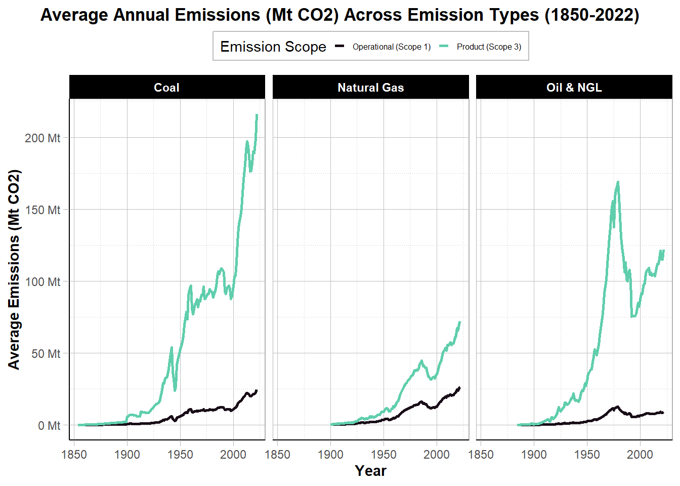
plot_2 <- ggplot(data = em_by_entity, aes(x = parent_type, y = emissions, fill = scope, color = parent_type)) +
  geom_bar(stat = "identity", linewidth = 0.8, alpha = 0.8) +
  facet_wrap(~commodity, ncol = 4) +
  scale_y_continuous(labels = label_number(suffix = "k Mt", scale = .001)) +
  scale_x_discrete(labels = c(
    "Nation State" = "Nation State",
    "State-owned Entity" = "State-owned",
    "Investor-owned Company" = "Investor-owned"
  )) +
  labs(
    title = "Cumlative Emissions (Mt CO2) Across Entity,
    Commodity, and Scope Types",
    y = "Total Emissions (Mt CO2)",
    fill = "Emission Scope",
    color = "Entity Type",
    x = "Entity Type"
  ) +
  theme_proj1() +
  theme(
    legend.position = "top",
    legend.direction = "horizontal",
    legend.title = element_text(
      size = 8,
      face = "bold"
    ),
    legend.box.background = element_rect(color = "white", linewidth = 0),
    legend.box.just = "left",
    legend.key = element_rect(color = 0, linewidth = 0),
    legend.spacing = unit(0.5, "mm"),
    legend.box.spacing = unit(1, "mm"),
    legend.key.spacing = unit(1, "mm"),
    panel.grid.major.x = element_blank(),
    axis.text.x = element_text(
      angle = 20
    )
  ) +
  scale_fill_viridis_d(
    option = "magma",
    begin = 0.1,
    end = 0.97,
    labels = c(
      "Scope 1" = "Operational (Scope 1)",
      "Scope 3" = "Product (Scope 3)"
    )
  ) +
  scale_color_viridis_d(
    labels = c(
      "Nation State" = "Nation State",
      "State-owned Entity" = "State-owned",
      "Investor-owned Company" = "Investor-owned"
    ),
    begin = 0.05,
    end = 0.6
  )

plot_2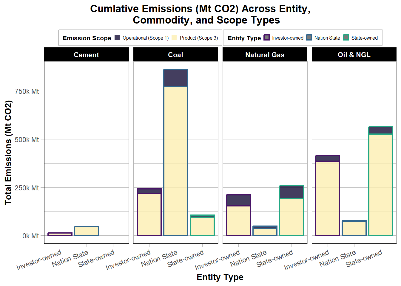
Discussion
(1-3 paragraphs) In the Discussion section, interpret the results of your analysis. Identify any trends revealed (or not revealed) by the plots. Speculate about why the data looks the way it does.
The analysis of Scope 1 and Scope 3 emissions across non-investor-owned entities reveals distinct trends based on commodity type. The first visualization, which tracks average emissions over time, shows that Scope 3 emissions vastly exceed Scope 1 emissions for all three commodities: Coal, Natural Gas, and Oil & NGL. This trend highlights that the majority of carbon emissions associated with these commodities come from downstream product use rather than from direct operations. This pattern is particularly evident for Coal and Oil & NGL, where Scope 3 emissions have sharply increased over the decades, reflecting the rising global demand for fossil fuels and their continued combustion for energy production.
The second visualization, a stacked bar plot comparing total emissions by entity type, further demonstrates this imbalance. State-owned entities and nation-states contribute significantly to emissions, particularly for Coal and Oil & NGL, where Scope 3 emissions dominate. This finding suggests that these non-investor-owned entities play a central role in global emissions, not just from production activities but also from the use of the products they extract and distribute. Cement, while included in the dataset, appears to have relatively low emissions in this comparison, likely because Scope 1 emissions (from production) are more relevant to cement than Scope 3 emissions.
A takeaway from these findings is that policies targeting only operational emissions (Scope 1) may be insufficient in addressing the full scope of carbon output. Since Scope 3 emissions drive the majority of the carbon footprint, regulatory efforts should focus not only on production-side interventions but also on end-use reductions, such as transitioning to renewable energy, carbon capture technologies, or stricter fuel consumption regulations. Additionally, the dominance of state-controlled entities in coal and oil production suggests that government policies and international agreements will be critical in shaping future emission trajectories.
One noticeable trend in the data is the persistent and growing dominance of Scope 3 emissions over time, particularly in Coal and Oil & NGL, despite major climate policies being introduced (there is a minor dropoff for oil but it has since picked back up). This suggests that efforts to curb emissions at the production level (Scope 1) have little effect on the demand for fossil fuels as it remains high, driving continued increases in consumer-side emissions. Additionally, state-owned entities and nation-states have played a larger role in Coal-related emissions, reinforcing the idea that government-controlled industries remain heavily invested in fossil fuel production.
These results align with broader trends in global climate policy discussions, where the emphasis is shifting toward full-lifecycle emissions accounting rather than just operational reductions. Future research could explore how specific national policies or corporate strategies have influenced these trends, particularly in major state-owned energy sectors. The dominance of state-controlled entities in coal and oil production suggests that government policies and international agreements will be critical in shaping future emission trajectories. The results also directly align with the motivation behind our team’s selection of this dataset because as Generation Z, we have grown up with the climate crisis as an ever-present reality and we can see that corporate accountability and government responsibility continue to be central themes in this crisis.
Presentation
Our presentation can be found here.
Data
Include a citation for your data here. See http://libraryguides.vu.edu.au/c.php?g=386501&p=4347840 for guidance on proper citation for datasets. If you got your data off the web, make sure to note the retrieval date.
References
List any references here. You should, at a minimum, list your data source.