UFO Sightings

Exploration

library(tidyverse)
library(skimr)
library(openxlsx)
library(scales)
library(janitor)
library(viridis)
library(dbscan)

Objective(s)

Project Topic: UFO Sightings

We believe this topic is important because it contributes to a better understanding of unexplained phenomena, helps in potential advancements in astronomy, and could encourage critical thinking and scientific exploration. Our final deliverable will be an interactive web app that allows people to input their zipcode or city to see UFO sightings near them.

Overall, there are three overarching questions we will be focusing on:

• How do geographical location and population density impact the frequency and duration of UFO sightings?

  • Are there discernible patterns or trends in UFO observations based on specific locations?

  • Is there any correlation between the region of sightings and the duration of the sightings?

  •  Is there any connection between the frequency of UFO sightings and population density?

•  How have the patterns of UFO sightings changed over historical timelines, and are they associated with any particular events?

  • Have the number of sightings fluctuated over time? 

  • Can any historical events or coincidental occurrences be related to a change in the amount or type of sightings?

• Are there any other factors that affect UFO sightings or interesting patterns?

  • Do the summary descriptions of sightings share any common themes or anomalies?

  • Does the time period (day vs night) or specific dates impact the likelihood of sightings?

  • Are there any patterns in the types of UFOs sighted in different locations and times?

Data collection and cleaning

ufo1 <- read_csv("data/nuforc_events.csv")

Rows: 110265 Columns: 13
── Column specification ────────────────────────────────────────────────────────
Delimiter: ","
chr  (6): City, State, Shape, Duration, Summary, Event_URL
dbl  (5): Year, Month, Day, Hour, Minute
dttm (1): Event_Time
date (1): Event_Date

ℹ Use `spec()` to retrieve the full column specification for this data.
ℹ Specify the column types or set `show_col_types = FALSE` to quiet this message.

ufo2 <- read_csv("data/ufo_data_nuforc.csv")

Rows: 1317 Columns: 13
── Column specification ────────────────────────────────────────────────────────
Delimiter: ","
chr  (9): posted, date, city, state, shape, duration, summary, images, img_link
dbl  (3): lat, lng, population
time (1): time

ℹ Use `spec()` to retrieve the full column specification for this data.
ℹ Specify the column types or set `show_col_types = FALSE` to quiet this message.

#cleaning the names before cleaning dataset 
ufo1_cleaned <- ufo1 |> 
  janitor::clean_names() |> 
  select(-event_time, -event_date) 

ufo2_cleaned <- ufo2 |> 
  janitor::clean_names() |> 
  select(-posted) |> 
  mutate(date = as.Date(date, "%m/%d/%Y")) |> 
  mutate(hour = hour(time), 
         minute = minute(time), 
         year = year(date), 
         month = month(date), 
         day = day(date))

#selecting only needed columns 
ufo2_cleaned <- ufo2_cleaned |> 
  select(-date, -time)

ufo2_cleaned <- ufo2_cleaned |> 
  mutate(year = ifelse(year > 23, paste0("19", year), paste0("20", year))) |> 
  mutate(year = as.numeric(year))

common_columns <- c("year", "month", "day", "hour", "minute", "city", "state", "shape", "duration", "summary") 

#merging 
merged <- bind_rows(ufo1_cleaned, ufo2_cleaned)

#recreating date 
merged$Date <- as.Date(paste
                       (merged$month, merged$day, merged$year, sep = "/"), 
                       format = "%m/%d/%Y")

#changing the month values to be abbrevs instead
merged <-merged |>
  mutate(month = recode(month, 
                        "01" = "Jan",
                        "02" = "Feb",
                        "03" = "Mar",
                        "04" = "Apr",
                        "05" = "May",
                        "06" = "June",
                        "07" = "July",
                        "08" = "Aug",
                        "09" = "Sep",
                        "10" = "Oct",
                        "11" = "Nov",
                        "12" = "Dec"))

#removing different variations of minutes in the duration column
remove_minutes_variations <- function(duration) {
  minutes_variations <- c("min", "mins", "minutes", "minute")
  duration <- gsub(paste(minutes_variations, collapse = "|"), "", duration, ignore.case = TRUE)
  return(duration)
}

#creating a function to turn all values in duration to minutes
to_minutes <- function(duration) {
  if (grepl("[~><-]", duration)) {
    return(duration)  # Keep such values as they are
  } else {
    # Extracting numeric values and their units
    numeric_value <- as.numeric(gsub("[^0-9]+", "", duration))
    unit <- tolower(gsub("[0-9]+", "", duration))
    
    # Use the remove_minutes_variations function to remove variations of "minutes"
    duration <- remove_minutes_variations(duration)
    
      # Converting all other values to minutes
      if (grepl("sec | Sec | secs | Secs | Seconds | Second | seconds | second", unit)) {
        return(round(numeric_value / 60, 3))
      } else if (grepl("hours | hour | Hour | Hours ", unit)) {
        return(round(numeric_value * 60, 3))
      } else {
        return(duration)  # Retaining strings and others as is
      }
    }
}

# Apply the to_minutes function to the 'duration' column of your dataframe
merged$duration <- sapply(merged$duration, to_minutes)

Data description

What are the observations (rows) and the attributes (columns)?

We have 111,582 rows and 17 variables.

Each row represents one specific UFO sighting, along with other characteristics about the sighting, such as the date, time, duration, summary, location, etc. The columns we will be focusing on are:

year: The year that the specific UFO sighting occurred.

month: The month in which the specific UFO sighting occurred.

day: The day on which the specific UFO sighting occurred. 

hour: The hour of the day at which the specific UFO sighting occurred.

minute: The minute of the day at which the specific UFO sighting occurred.

city: The US city in which the specific UFO sighting occurred.

state: The US state in which the specific UFO sighting occurred.

shape: The shape that the UFO appeared to be in to the person it was seen by.

duration: The duration of time that the UFO was seen for. 

summary: The summary of the UFO sighting provided by the person who saw it. 

event_url: A link to the posting about the UFO sighting.

images: An indication of whether the specific UFO sighting has an associated or not. The values are either ‘yes’, ‘no’ or NA.

img_link: A link to the image associated with the specific UFO sighting. 

lat: The exact latitude of where the UFO sighting occurred.

lng: The exact longitude of where the UFO sighting occurred. 

population: The population of the city in which the UFO sighting occurred.

date: The full date of the UFO sighting.

Why was this dataset created?

The National UFO Reporting Center established this dataset to collect, verify, and archive accounts of potential UFO sightings from diverse sources. The creation of this dataset promotes transparency by making UFO-related data publicly accessible and encourages further research and understanding of UFO phenomena.

Who funded the creation of the dataset?

The National UFO Reporting Center was founded in 1974 by Robert J. Gribble, a UFO investigator. 

What processes might have influenced what data was observed and recorded and what was not?

The main means to report sightings since 1994 has been the website. However, before reports were made through phone calls and mail. The type of reporting mechanisms available, and who has access to them, could have influenced who was able to report the sighting and what details they could include. Furthermore, the extent of public awareness and belief in UFO sightings could have played a role too; periods of higher public interest or notable events might have led to more reporting, or certain regions where people are more likely to believe in UFOs could have reported more sightings. Lastly, because the Center ensures anonymity of the person reporting, it is possible that more people felt comfortable reporting. 

What preprocessing was done, and how did the data come to be in the form that you are using?

We got both our datasets from data world (linked below under sources), and they got the data from the National UFO Reporting Center. During the preprocessing, the authors added geocoding data such as latitude, longitude and population of city to the ufo2 dataset. The time variable was also broken into hours and minutes for the ufo1 dataset.

If people are involved, were they aware of the data collection and if so, what purpose did they expect the data to be used for?

Given that the primary data comes from individuals who reported their sightings to the National UFO Reporting Center, we can assume that these individuals were aware that their reports were being collected as data. The center also has a policy of guaranteed anonymity, which suggests that informants were aware of their part in the data collection process. The Center also seems to be very open about their policy surrounding collected data, so it is likely that individuals expected their reports to be used in research and public knowledge. 

Data limitations

• All of the data we have is self-reported, which means that there are several inconsistencies within the data, especially in text columns such as duration and summary. This means that it is difficult to standardize the data in these columns.

• Another potential problem arises from joining the two datasets that we have. Some columns that we will be using, such as population, are only present in one dataset, which led to a lot of NA values after we performed our join.

• The main topic surrounding the dataset is UFOs, which can be seen by many as superstitious. Only people who believe in UFOs would have reported to the website, even if others had seen similar sightings. This means that we have an unrepresentative and biased dataset.

Exploratory data analysis

Perform an (initial) exploratory data analysis.

#Exploring which cities have the most sightings:
#Count per city
explore_city <- merged |>
  group_by(city) |>
  summarise(
    count = n()
  ) |>
  arrange(-count) |> 
  slice(1:10)

explore_city

# A tibble: 10 × 2
   city        count
   <chr>       <int>
 1 Seattle       640
 2 Phoenix       634
 3 Las Vegas     521
 4 Portland      514
 5 San Diego     434
 6 Los Angeles   430
 7 Chicago       368
 8 Houston       360
 9 Tucson        341
10 Miami         314

ggplot(explore_city, aes(x = reorder(city, -count), y = count, fill = reorder(city, -count))) +
         geom_bar(stat = "identity") +
  theme_minimal() +
  labs(x = '',
       y = "Number of UFO Sightings",
       fill = '',
       title = "Which Cities Have the Most Sightings?") +
  theme(axis.text.x = element_blank())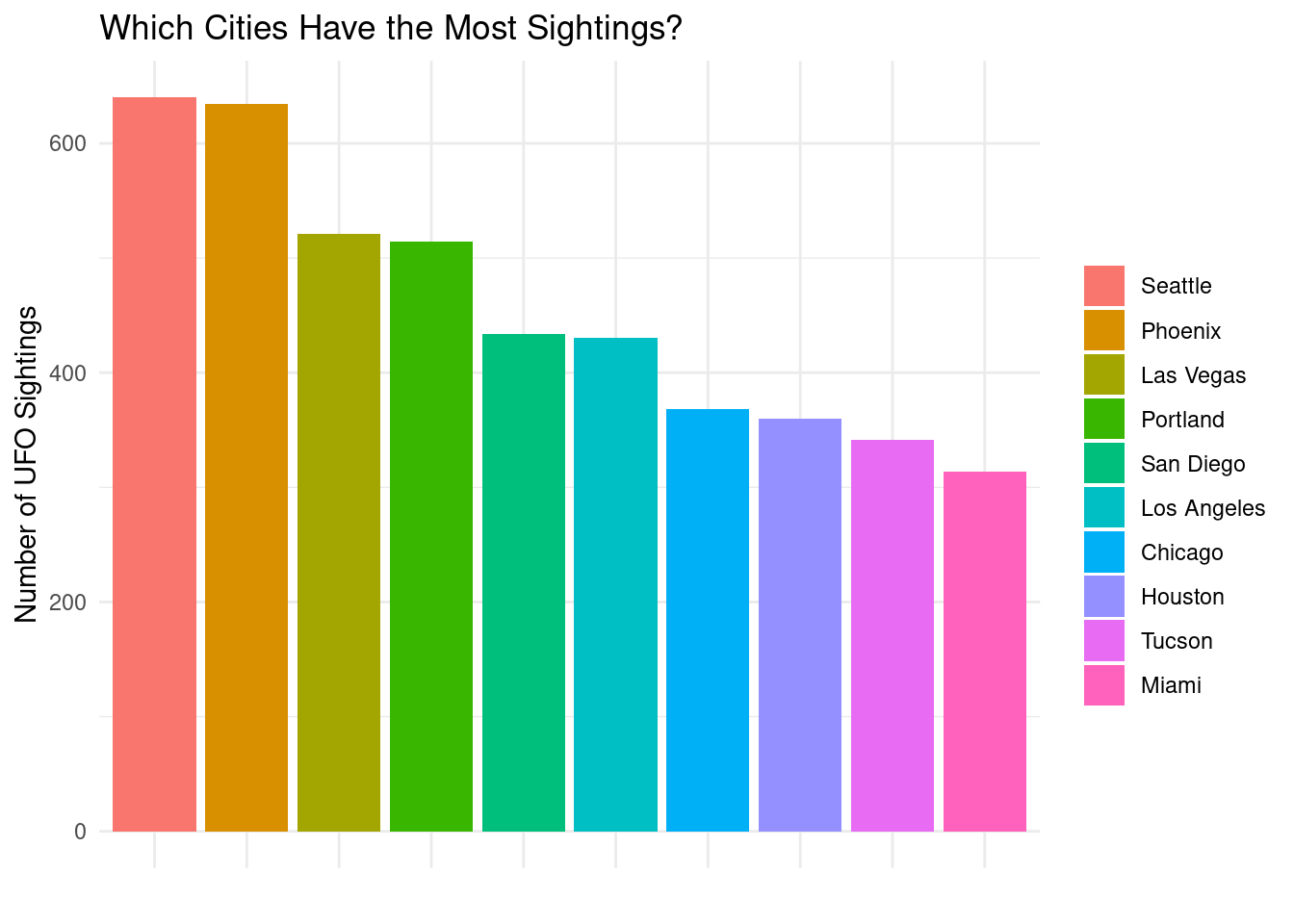

#Are there certain months with more sightings?
explore_month <- merged |>
  select(year, month) |>
  group_by(month, year) |>
  summarise(
    count = n()
  ) |>
  arrange(-count) |> 
  slice(1:10) |>
  mutate(
    year = factor(year, levels = sort(unique(year))),
    month = factor(month, levels = c("Jan",
                                     "Feb",
                                     "Mar",
                                     "Apr",
                                     "May",
                                     "Jun",
                                     "Jul",
                                     "Aug",
                                     "Sep",
                                     "Oct",
                                     "Nov",
                                     "Dec"))) |>
  #arranged by each year and months
   arrange(year, month) |>
  drop_na()

`summarise()` has grouped output by 'month'. You can override using the
`.groups` argument.

ggplot(explore_month, aes(x = month,
                              y = count,
                              fill = month)) +
  geom_boxplot() + 
  theme_minimal() +
  labs(x = 'Month',
       y = "UFO Sightings",
       title = "How do UFO sightings vary across months?",
       subtitle = "Shown across years",
       fill = '')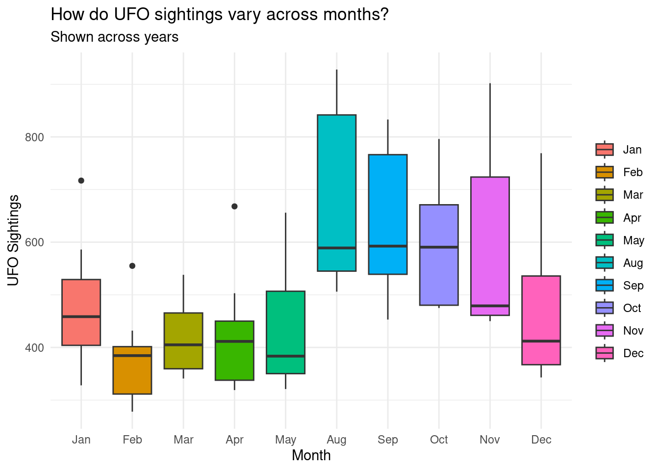

explore_occurance <- merged |>
  filter(!is.na(year) & year >= 1800) |>
  group_by(year) |>
  summarise(count = n())

ggplot(explore_occurance, aes(x = year, y = 1, fill = count)) +
  geom_tile() +
  labs(title = "UFO Sightings Over the Years",
       x = "Year",
       y = "") + 
  theme_minimal() +
  scale_color_viridis(discrete = TRUE, option = "C")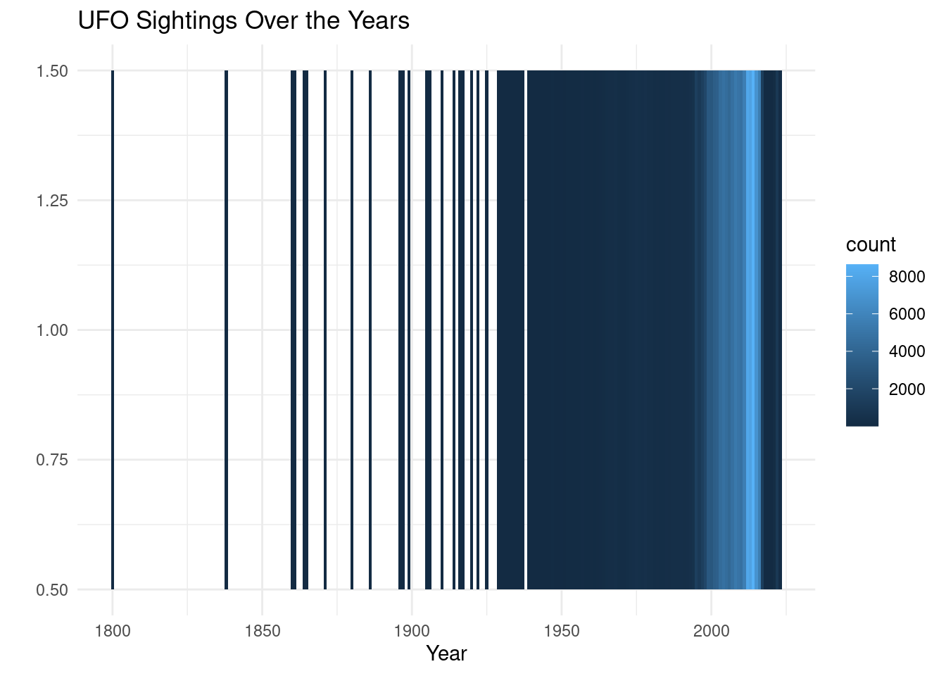

explore_population <- merged |>
  select(city, state, population) |>
  filter(!is.na(population)) |>
  mutate(
    population_range = case_when(
      population < 30000 ~ "Not populated (Low)",
      population >= 30000 & population <= 90000 ~ "Slightly populated (Moderate)",
      population > 90000 & population <= 1000000 ~ "Intermediate (High)",
      population > 1000000 ~ "Highly populated (Very High)"
    )
  ) 

city_sightings <- merged |>
  group_by(city) |>
  summarise(count = n()) |>
  arrange(desc(count))


combined_data <- merge(explore_population, city_sightings, by = "city")

ggplot(combined_data, aes(x = population_range, y = count, fill = population_range)) +
  geom_bar(stat = "identity") +
  labs(
    title = "UFO Sightings vs. Population Density by City",
    x = "Population Range",
    y = "Number of UFO Sightings",
    fill = "Population Range"
  ) +
  theme_minimal() +
  theme(axis.text.x = element_blank())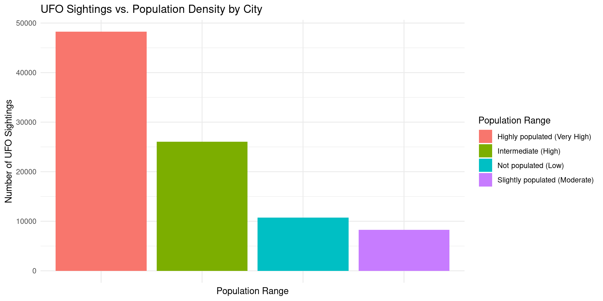

coords <- ufo2_cleaned[, c("lat", "lng")]

coords <- na.omit(coords)

# Perform DBSCAN clustering
db <- dbscan(coords, eps = 0.1, minPts = 5)  # Use 'minPts' instead of 'MinPts'

# Add cluster labels to the original data
ufo2_cleaned$cluster <- db$cluster

# Plot the clusters
ggplot(ufo2_cleaned, aes(x = lng, y = lat, color = factor(cluster))) +
  geom_point() +
  labs(title = "UFO Sightings Clusters", color = "Cluster") +
  theme_minimal()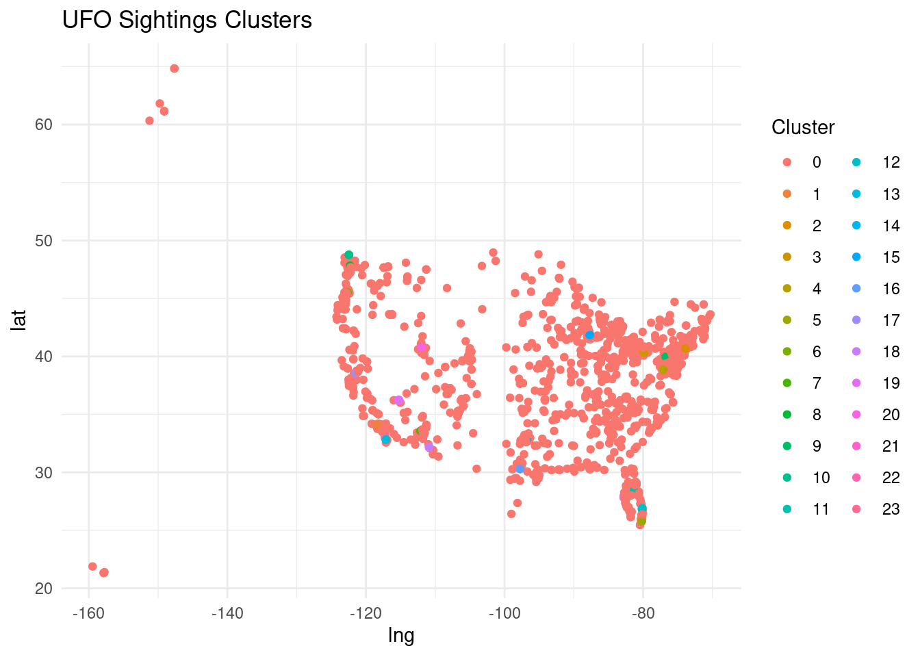

#
# Extract latitude and longitude columns from ufo2_cleaned
coords <- ufo2_cleaned[, c("lat", "lng")]

# Perform DBSCAN clustering
db <- dbscan(coords, eps = 0.1, minPts = 5)

# Add cluster labels to the ufo2_cleaned data
ufo2_cleaned$cluster <- db$cluster

# Define population ranges
ufo2_cleaned <- ufo2_cleaned %>%
  mutate(
    population_range = case_when(
      population < 20000 ~ "Not populated (Low)",
      population >= 20000 & population <= 60000 ~ "Slightly populated (Moderate)",
      population > 60000 & population <= 100000 ~ "Intermediate (High)",
      population > 100000 ~ "Highly populated (Very High)"
    )
  )

# Create a summary of the count of sightings per cluster and population range
cluster_population_data <- ufo2_cleaned %>%
  group_by(cluster, population_range) %>%
  summarise(count = n())

`summarise()` has grouped output by 'cluster'. You can override using the
`.groups` argument.

# Create a bar plot with population range labels
ggplot(cluster_population_data, aes(x = reorder(population_range, -count), y = count, fill = factor(cluster))) +
  geom_bar(stat = "identity") +
  labs(
    title = "UFO Sightings vs. Population Density by Cluster",
    x = "Population Range",
    y = "Number of UFO Sightings",
    fill = "Cluster"
  ) +
  theme_minimal() +
  theme(axis.text.x = element_text(angle = 45, hjust = 1))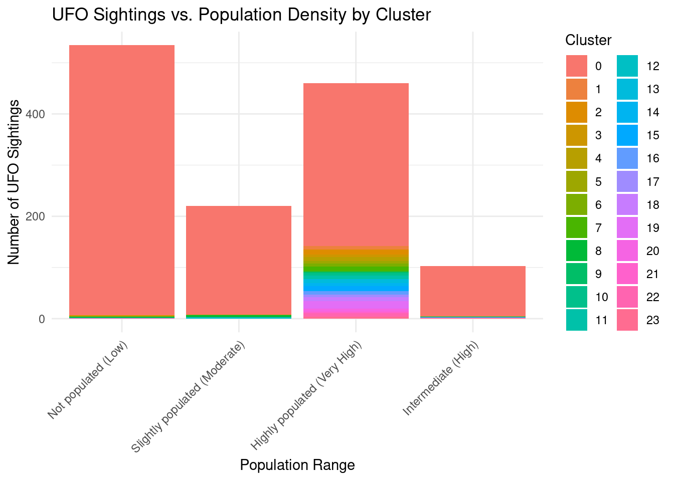

#write.csv(merged, "~/fa23_project/project-elegant-charmander/data/ufo_merged_data.csv", row.names = FALSE) 

Questions for reviewers

List specific questions for your peer reviewers and project mentor to answer in giving you feedback on this phase.

• How can we handle the textual data in the duration column? We have converted most of the values to minutes for example, if it says 30 minutes or 1 hour. However, it also has some text like “All night”. For values like these, it is bad practice to convert these to the amount of time we assume all night to be? Furthermore, some values are ranges such as 10-15 minutes. For these, should we calculate the average?

• For our final deliverable, we are planning to create an interactive web app that allows users to input their city or zipcode to be able to see UFO sightings near them. Are there any packages you think would be useful for us to use for this? 

• Currently we have three main research questions, with some questions we’ll be exploring for each. Do you think our scope is reasonable, or do we need to narrow/broaden our questions? In the case where you think we should change, is there a certain question from our list that you think would be most interesting?

• Are we allowed to incorporate physical deliverables, such as a poster or pamphlet, into our presentation to make it more interactive?

• One dataset only has US states, and the second one has mostly US states, but also a few international locations. During our exploration, we saw that most UFO sightings were in US states, so is it reasonable to narrow our scope to only look at UFO sightings in the US?

Sources Used:

National UFO Reporting Center. NUFORC. (2023, October 28). https://nuforc.org/

UFO data NUFORC - dataset by CK30. data.world. (2021, August 23). https://data.world/ck30/ufo-data-nuforc

National UFO Reporting Center Reports - dataset by khturner. data.world. (2017, April 25). https://data.world/khturner/national-ufo-reporting-center-reports