The primary objective of this project is to develop a Correlation Analysis Tool and deliver a comprehensive analysis of correlations between various movie-related parameters, including film length, IMDB rating, distributing studio, genre, and worldwide gross. This analysis will be facilitated through the following key deliverables:
Correlation Analysis Tool:Create a Shiny web app for interactive parameter selection and correlation visualization.
Visual Insights: Develop scatter plots, correlation matrices, and trend lines within the app to highlight key correlations and provide valuable insights.
Summary Report: Generate a report summarizing major findings, significant correlations, and insights from the analysis to offer a comprehensive view of movie parameter relationships.
The dataset was generated as a result of a data categorization project organized by CrowdFlower. The primary objective of this project was to compile data on the ten most popular movies for each year within the time frame of 1975 to 2015. The dataset contains 410 data rows, representing a substantial selection of popular movies spanning four decades.
This dataset provides a rich and comprehensive view of popular movies from different genres and time periods. It serves as a valuable resource for analyzing trends in the movie industry, evaluating movie ratings, and examining the financial performance of these movies over the specified 40-year period. For researchers, analysts, and enthusiasts interested in the evolution of the film industry over these decades, this dataset offers a robust foundation for conducting insightful analyses and drawing meaningful conclusions.
Data Cleaning
The raw data obtained from the source was already cleaned and required minimal additional cleaning for analysis. The cleaning process primarily focused on ensuring the data was in a suitable format and addressing any potential issues:
Missing Values: The dataset was checked for missing values. Fortunately, there were no significant missing values, and any that were present were appropriately labeled as “NA.”
Data Type Conversion: Some columns required data type conversion for analysis. For instance, “worldwide_gross” and “rating” columns were converted from character to numeric types, while “year” and “rank_in_year” were converted to integer types.
Special Characters: In the “worldwide_gross” and “rating” columns, special characters, such as dollar signs and commas, were removed to ensure numeric data types could be applied. For “rating,” we extracted the numeric part.
As the data was already cleaned, the code used for cleaning was straightforward and did not involve extensive transformations. The code for data curation and cleaning, as previously provided, was applied to ensure that the data was in an analysis-ready format.
── Attaching core tidyverse packages ──────────────────────── tidyverse 2.0.0 ──
✔ dplyr     1.1.2     ✔ readr     2.1.4
✔ forcats   1.0.0     ✔ stringr   1.5.0
✔ ggplot2   3.4.3     ✔ tibble    3.2.1
✔ lubridate 1.9.2     ✔ tidyr     1.3.0
✔ purrr     1.0.2
── Conflicts ────────────────────────────────────────── tidyverse_conflicts() ──
✖ dplyr::filter() masks stats::filter()
✖ dplyr::lag()    masks stats::lag()
ℹ Use the conflicted package (<http://conflicted.r-lib.org/>) to force all conflicts to become errors
# Download the file manually download.file("https://drive.google.com/uc?export=download&id=1CxuUp_pjOKZXrgZ6JkW4n-kUMUyrhavP", "blockbusters.csv")# Specify the column typescolumn_types <-cols(Main_Genre =col_character(),Genre_2 =col_character(),Genre_3 =col_character(),rating =col_character(),studio =col_character(),title =col_character(),worldwide_gross =col_character(),imdb_rating =col_double(),length =col_double(),rank_in_year =col_double(),year =col_double())# Read the CSV fileblockbusters <-read_csv("blockbusters.csv", col_types = column_types)#Minimal cleaning# Convert "worldwide_gross" to numericblockbusters$worldwide_gross <-as.numeric(gsub("\\$", "", gsub(",", "", blockbusters$worldwide_gross)))# Clean the "rating" column (assuming you want to keep only numeric part)blockbusters$rating <-as.numeric(gsub(".*?([0-9.]+).*", "\\1", blockbusters$rating))
Warning: NAs introduced by coercion
# Optionally, convert "year" and "rank_in_year" to integersblockbusters$year <-as.integer(blockbusters$year)blockbusters$rank_in_year <-as.integer(blockbusters$rank_in_year)# Check for any remaining issuesglimpse(blockbusters)
The dataset includes the following key attributes, making it well-suited for comprehensive analyses related to the movie industry:
Observations and Attributes:
Observations (Rows): 437
Attributes (Columns): 11
Main_Genre: The primary genre of the movie.
Genre_2: Additional information about the genre.
Genre_3: Further genre information; some entries are NA (Not Available).
imdb_rating: The IMDb rating of the movie.
length: The duration of the movie in minutes.
rank_in_year: The rank of the movie among the top movies in its respective year.
rating: The MPAA rating of the movie (e.g., PG-13, PG, R).
studio: The studio that produced/distributed the movie.
title: The title of the movie.
worldwide_gross: The worldwide gross box office receipts for the movie.
year: The year in which the movie was released
Creation of the Dataset
Purpose: The dataset was created to gather information about the ten most popular movies for each year over a span of 40 years (1975-2015).
Funding: The dataset was generated as a result of a data categorization project organized by CrowdFlower.
Influencing Factors on Data Collection: The data collection was influenced by a data categorization job, where the crowd was asked to find information about the most popular movies for each year. This likely influenced the inclusion of popular movies but might have excluded less well-known films.
Preprocessing and Data Form:
Preprocessing: The data underwent categorization, likely involving tasks such as extracting movie titles, gathering genre information, obtaining run time, ratings, and box office receipts.
Data Form: The data is organized in tabular form with rows representing individual movies and columns containing information about the movies.
Awareness and Purpose: It’s not explicitly mentioned whether the people involved were aware, but given it was a crowd-based task, participants likely knew they were contributing to a movie information dataset.The data was likely collected with the purpose of creating a comprehensive resource for analyzing movie industry trends, ratings, and financial performance over the specified 40-year period. Participants might have expected the data to be used for research and analysis in the field of movie studies or related domains. ##
Data limitations
A significant concern is the impact of changing movie ticket prices over the past 50 years. In 1975, a successful movie might have generated similar box office revenue to what a mediocre movie did in 2010. Hence, comparing box office receipts directly without accounting for inflation can result in misleading conclusions and an inaccurate evaluation of a movie’s performance. To ensure a fair and accurate assessment, it is essential to adjust for inflation when comparing box office earnings across different time periods.
Other potential problems could be:
Sample Bias: The dataset represents the most popular movies for each year. This could introduce bias, as it focuses on a specific subset of movies. The analysis should acknowledge this and consider potential generalizability issues.
Temporal Trends: The dataset spans several decades, and the movie industry has evolved significantly over time. It’s important to consider how temporal trends and industry changes might affect the analysis and conclusions.
Bias in Rating Systems: The IMDb rating and other rating systems may introduce bias, as they are subject to manipulation and can be influenced by various factors, including user demographics.
Exploratory data analysis
library(tidyverse)library(reshape2)library(scales)# Download the file manually download.file("https://drive.google.com/uc?export=download&id=1CxuUp_pjOKZXrgZ6JkW4n-kUMUyrhavP", "blockbusters.csv")# Specify the column typescolumn_types <-cols(Main_Genre =col_character(),Genre_2 =col_character(),Genre_3 =col_character(),rating =col_character(),studio =col_character(),title =col_character(),worldwide_gross =col_character(),imdb_rating =col_double(),length =col_double(),rank_in_year =col_double(),year =col_double())# Read the CSV file blockbusters <-read_csv("blockbusters.csv", col_types = column_types)# Display the structure of the datasetstr(blockbusters)
# Summary statistics for numerical variablessummary(blockbusters)
  Main_Genre          Genre_2            Genre_3           imdb_rating
 Length:437         Length:437         Length:437         Min.   :4.400
 Class :character   Class :character   Class :character   1st Qu.:6.500
 Mode  :character   Mode  :character   Mode  :character   Median :7.100
                                                          Mean   :7.077
                                                          3rd Qu.:7.700
                                                          Max.   :9.000
     length       rank_in_year       rating             studio
 Min.   : 27.0   Min.   : 1.000   Length:437         Length:437
 1st Qu.:103.0   1st Qu.: 3.000   Class :character   Class :character
 Median :118.0   Median : 6.000   Mode  :character   Mode  :character
 Mean   :119.9   Mean   : 5.524
 3rd Qu.:134.0   3rd Qu.: 8.000
 Max.   :201.0   Max.   :10.000
    title           worldwide_gross         year
 Length:437         Length:437         Min.   :1975
 Class :character   Class :character   1st Qu.:1986
 Mode  :character   Mode  :character   Median :1997
                                       Mean   :1997
                                       3rd Qu.:2008
                                       Max.   :2018
# Check for missing valuesany(is.na(blockbusters))
[1] TRUE
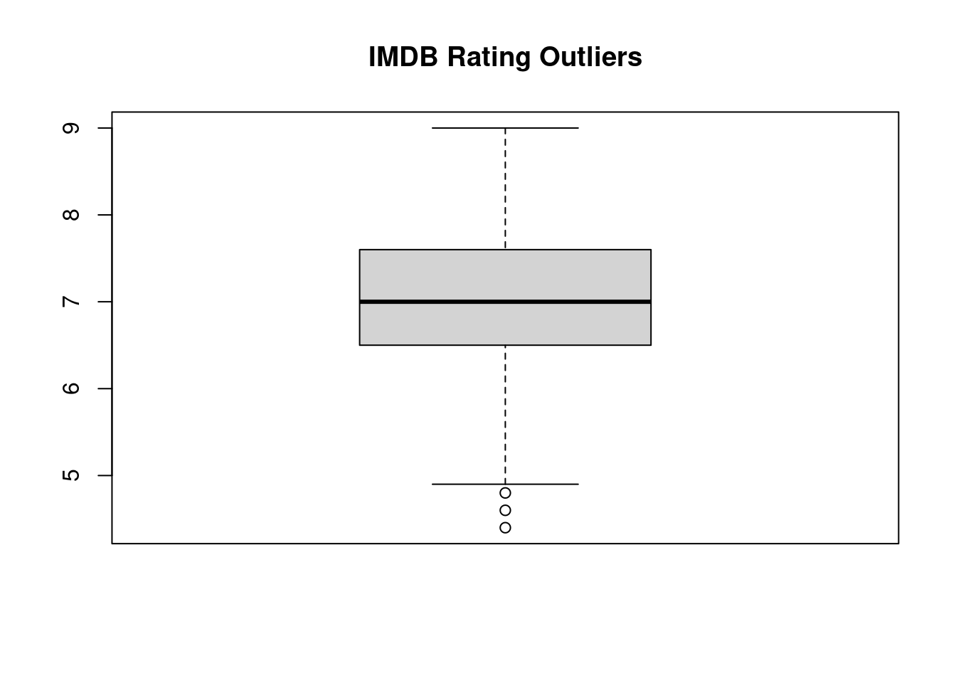
# Remove rows with missing values, if necessaryblockbusters <- blockbusters %>%drop_na()# Check for outliers in numerical variablesboxplot(blockbusters$imdb_rating, main ="IMDB Rating Outliers")
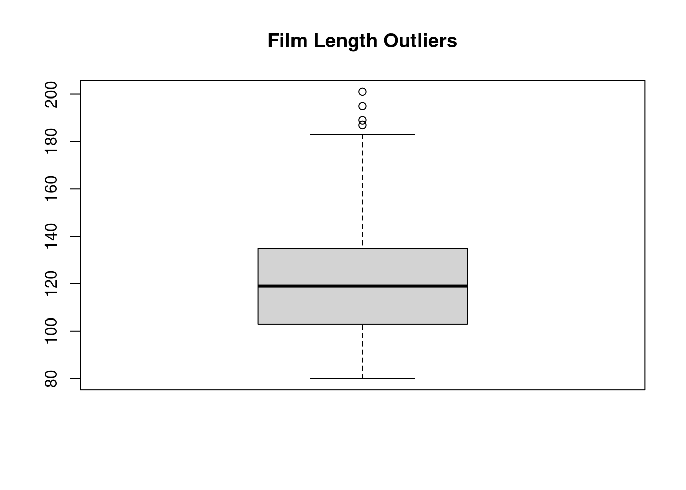
boxplot(blockbusters$length, main ="Film Length Outliers")
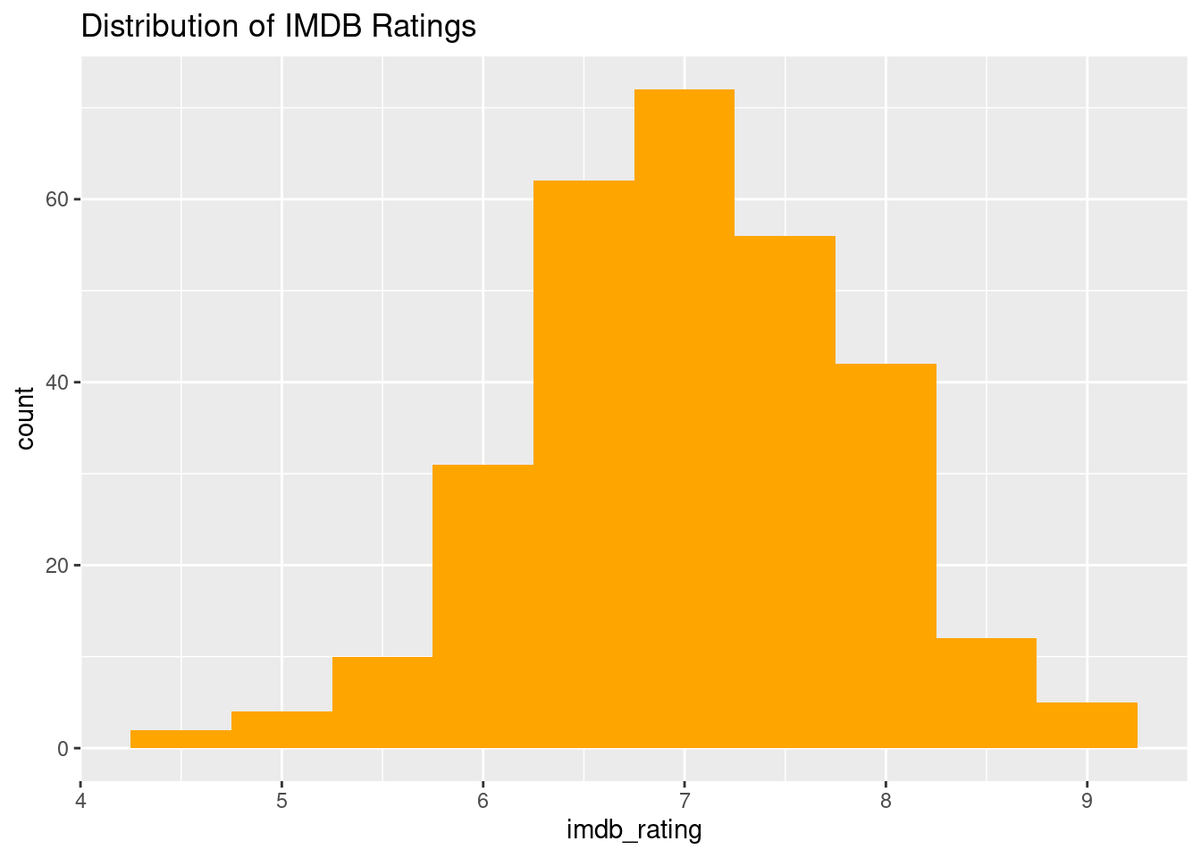
# Histogram of IMDB Ratingsggplot(blockbusters, aes(x = imdb_rating)) +geom_histogram(binwidth =0.5, fill ="orange") +labs(title ="Distribution of IMDB Ratings")
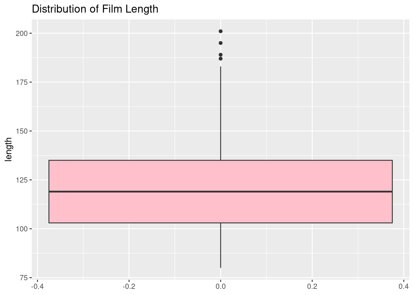
# Boxplot of Film Lengthggplot(blockbusters, aes(y = length)) +geom_boxplot(fill ="pink") +labs(title ="Distribution of Film Length")
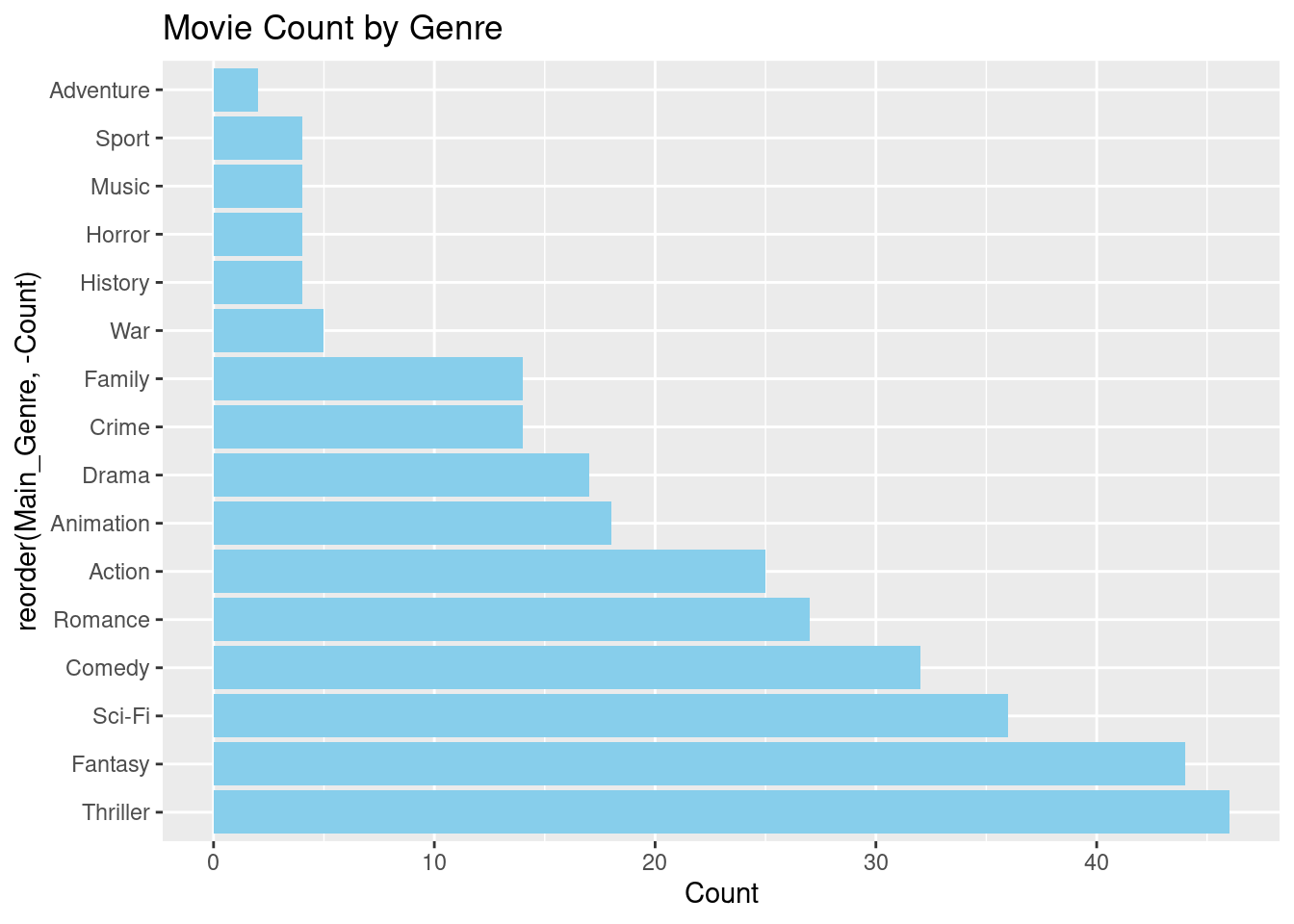
# Count of movies by genregenre_count <- blockbusters %>%group_by(Main_Genre) %>%summarise(Count =n()) %>%arrange(desc(Count))# Bar plot of movie count by genreggplot(genre_count, aes(x =reorder(Main_Genre, -Count), y = Count)) +geom_bar(stat ="identity", fill ="skyblue") +coord_flip() +labs(title ="Movie Count by Genre")
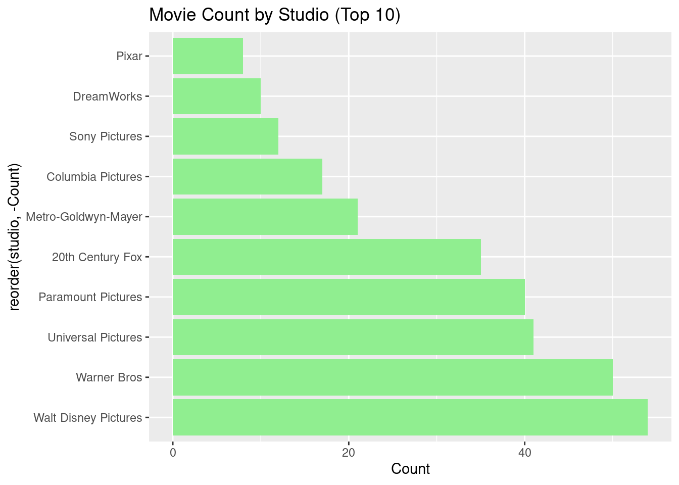
# Count of movies by studiostudio_count <- blockbusters %>%group_by(studio) %>%summarise(Count =n()) %>%arrange(desc(Count)) %>%top_n(10)# Bar plot of movie count by studioggplot(studio_count, aes(x =reorder(studio, -Count), y = Count)) +geom_bar(stat ="identity", fill ="lightgreen") +coord_flip() +labs(title ="Movie Count by Studio (Top 10)")
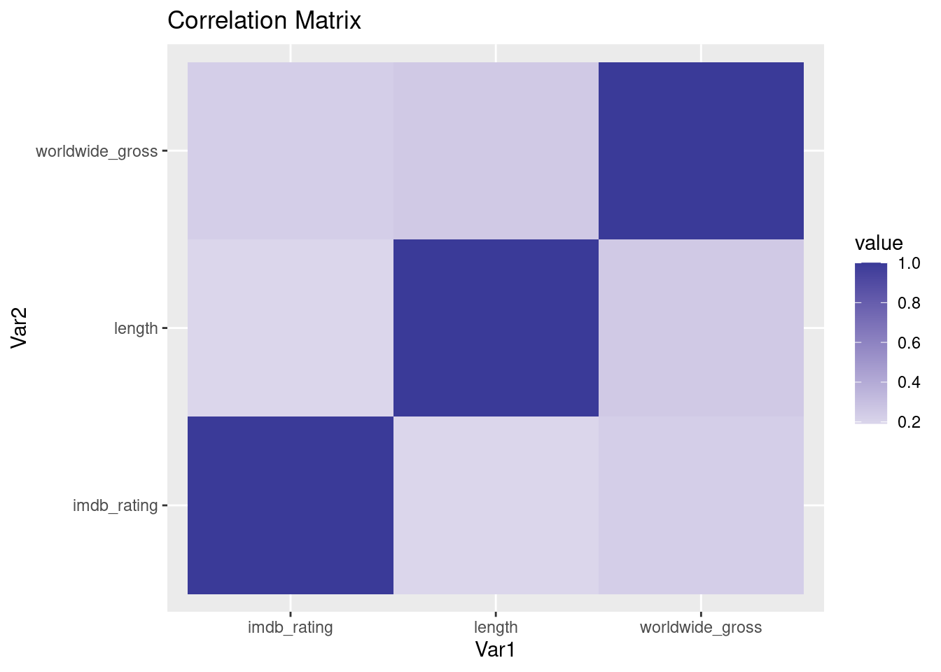
# Remove commas and dollar signs from "worldwide_gross" and convert to numericblockbusters$worldwide_gross <-as.numeric(gsub("[\\$,]", "", blockbusters$worldwide_gross))# Calculate the correlation matrix (with automatic handling of missing values)correlation_matrix <-cor(select(blockbusters, imdb_rating, length, worldwide_gross))corr_matrix_melted <-melt(correlation_matrix)corr_plot <-ggplot(corr_matrix_melted, aes(Var1, Var2, fill = value)) +geom_tile() +scale_fill_gradient2() +labs(title ="Correlation Matrix")# Display the heatmapprint(corr_plot)
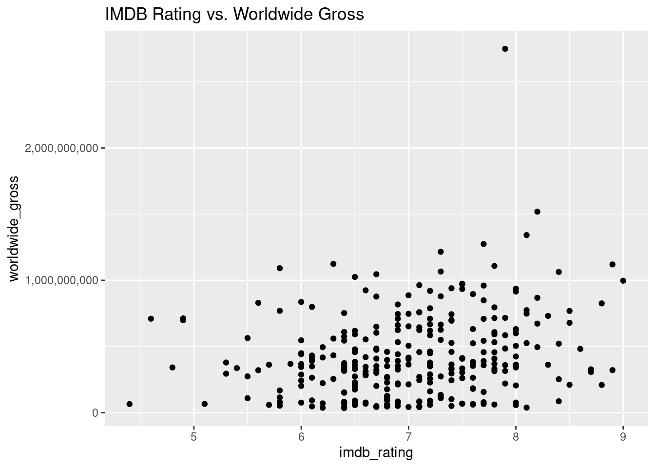
# Remove commas and dollar signs from "worldwide_gross" and convert to numericblockbusters$worldwide_gross <-as.numeric(gsub("[\\$,]", "", blockbusters$worldwide_gross))# Scatter plot to explore relationships (e.g., IMDB rating vs. Worldwide Gross)ggplot(blockbusters, aes(x = imdb_rating, y = worldwide_gross)) +geom_point() +labs(title ="IMDB Rating vs. Worldwide Gross") +scale_y_continuous(labels = comma)
Questions for reviewers
A few questions we have:
Have all potential limitations and issues associated with the Blockbuster dataset been identified and addressed?
Do you have any recommendations for mitigating or addressing the limitations of the dataset?
What kinds of parameters do we need to put on our interactive website for users to input?
Does the initial exploratory data analysis (EDA) provide meaningful insights into the Blockbuster dataset, and is it aligned with the project’s objectives?
Are there specific relationships, patterns, or trends in the data that you believe should be further explored or visualized during EDA?
Considering the characteristics and insights from the dataset’s initial exploration, what are the next logical steps for the project?
Is the project’s documentation clear, well-organized, and easy to follow, and are there any sections or aspects that require additional explanations or clarifications?