Go To:
Home Page
Milestone 4
Milestone 3: Maze Exploration Algorithm
Goals:
In simulation and in real life, we must:
- Create a working algorithm that facilitates maze exploration.
- Create an indicator that shows the robot is done, i.e. the robot has explored everything that is explorable.
In simulation:
Team members:
- Yonghun Lee, Logan Horowitz
Materials Used:
- Java
- Arduino Sketch
- Robot/Arduino
Depth First Search
We decided that the Depth First Search(DFS) is the most appropriate algorithm to start with. Here is our logic behind our decision:
- The primary goal of the maze exploration is to explore everywhere reachable to collect information about walls and treasurers on each grid, which can only be found either directly on the grids or in the vicinity of them.
- The time cost of turning at the intersections is high.
- Consequently, it is preferable to make an exhaustive search on its first exploration through a remote grid from the starting point without deviating from its straight path.
- DFS is very memory-efficient. The algorithm only requires one array of 20 grids that can hold every information necessary—(x,y) coordinate, walls, treasurers, and backpointers.
- Note: We wrote DFS algorithm in Java. In fact, the optimal language to use is C or C++, because the Arduino language is most compatible with them. Java is simply the most accessible language to the team members. And also, we felt Java’s object-orientated nature provides the easiest way to try out new ideas and its GUI provides the excellent platform to visualize the simulation. The basic structure of DFS is as followed. DFS uses stack data structure. As the robot travels, all adjacent nodes that are not blocked by the wall are added to the stack, a list of grid that the robot must travel. The robot stops when the stack is empty—in other words, when there is no more reachable nodes and all of the maze has been explored.
// Depth First Search - Basic Structure
public class dfs {
    Stack s= (u);                      // The list of grids that have to be visited
    while (s is not empty) {           // If the stack is empty, the robot is done!
        u= s.pop();                    // Next target grid is the topmost grid on stack
        if (u is not visited)
            visit u;
        for (Neighbors of u) {         // Add the neighbor grids of the current location to the stack.
            s.push(u);
        }
    }
    return;
}
Some of initializations and definitions should be clarified:
- Grid
/** 5 by 4 array is initialized. (row, column) is reversed to represent
* (x,y). (Ex. (row 2, column 3) -> (x,y) = (3,2). X,Y coordinate origin is
* at the top left. The robot's starting position is (x,y) = (3,4) */
public void gridInit() {
	grid= new Node[5][4];
	for(int i= 0; i < 5; i++) {
		for (int j= 0; j < 4; j++) {
			grid[i][j]= new Node(null, false, false, j, i);
		}
	}
}
 2. Wall
/** User-input maze. Decimal representative of wall location on each grid by
	 * 4bit binary number (msb)'(W)(E)(S)(N)'(lsb) */
public int[][] mazeInput1= new int[][] {
	{9,1,3,5},
	{8,6,13,12},
	{12,11,6,12},
	{8,3,7,14},
	{10,3,3,7}
};
- Node: In the Arduino language, we will implement unsigned 16 bit integer for each array element. In our simulation on Java, we created a Node object that contains the following information. *isSpecial indicates a node which we do more calculations on than non-special nodes. It is used later for backtracking algorithm.
/** Each grid contains the following information */
public class Node {
	private Node bckPntr;
	private boolean visited;
	private boolean isSpecial;
	public int x;
	public int y;
}
The key points of the algorithm are as followed:
- We add new target grids whenever we move onto the new grid. Stack is Last-In-First-Out data structure. Because we want the robot to go straight if possible, we first check and add its east and west neighbor grids, and add the grid the robot faces the last.
- Direction the robot is facing should be found simply by comparing the grid number of the new grid and the previous grid. If there is a wall on north side of its current direction, it will turn to move onto the other adjacent grid.
- We should always be aware of the boundary walls! They should be checked whenever the robot is on grid with x= 0 or 3/ y=0 or 4.
/** Check the neighbors of the grid, except for the grid from which the robot comes from.
 * (Direction tells us where the robot is coming from. The grid that the robot
 * is facing is checked first */
private List<Node> getPath(Node current) {
	List<Node> paths= new LinkedList<Node>();
	int directx= current.x - current.bckPntr.x;  // If it is 1, the robot is heading West
	int directy= current.y - current.bckPntr.y;  // If it is 1, the robot is heading South
	if (directx == 1) {  // Faces East
		if (maze[current.y][current.x].charAt(1) == '0') paths.add(grid[current.y][Math.min(3, current.x + 1)]);
		if (maze[current.y][current.x].charAt(3) == '0') paths.add(0, grid[Math.max(0, current.y - 1)][current.x]);
		if (maze[current.y][current.x].charAt(2) == '0') paths.add(0, grid[Math.min(4, current.y + 1)][current.x]);
	}

	/*.......... Cases for facing West, North, and South.................*/
	return paths;
}
- The robot cannot always move onto an adjacent node, as it will inevitably hit the end-grid, whose neighbors either have already been visited or blocked by walls.
- The stack will then pop a grid to give robot a new target that is remote from the current location (the grid that has been added on its way to this location). DFS then backtraces to the remote grid by using the backpointers to backtrack its previous path until it reaches there.
/** Backtracking using Backpointers */
while (!isPathOpen(position, u)) {
    prev= position;
	position= position.bckPntr;
	path.add(position);
}
//The robot is finally at the adjacent grid of the target grid!
u.bckPntr= position;
position= u;
This is the part where we can find the most apparent inefficiency of DFS. DFS cannot intelligently find its way to a remote target grid, because all the information it stores is the backpointer of each grid (this is unfortunately why DFS is very memory efficient!).
Here’s an example of maze that demonstrates this inefficiency in backtracking. If we use a regular backpointer method for backtracking, the robot chooses a non-ideal path to get to the remote target grid.
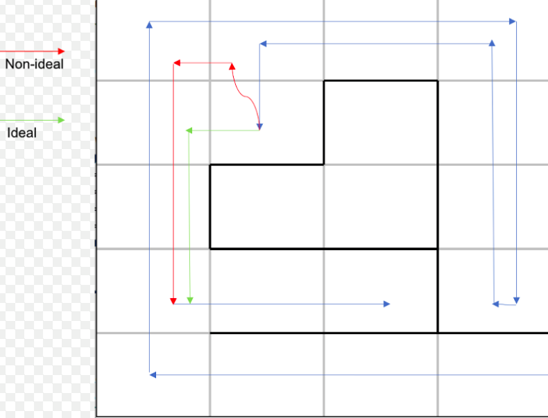
We tried to improve DFS’ regular backtracking method by calculating the Manhattan distance between each neighboring grid and the target grid whenever necessary (a grid whose isSpecial value is true!), and choose the one that has the shortest distance, instead of relying on the backpointers.
- Note: When do we make a grid ‘special’? We do so whenever the grid is popped off of stack as a remote target. And also, we mark a grid special, when we add its neighbors to stack and find that it has more than one reachable neighbors. The ones that are not-special are mostly those whose path are open only in one direction. When backtracking, the robot does not have to look into their neighbors, because the only way is through its pre-determined backpointers. Remember, our goal is to minimize unnecessary calculation and memory consumption.
for (Node n: neighbors) {
    int distance= (Math.abs(n.x-u.x)) + (Math.abs(n.y-u.y));
    if (distance < temps && n != prev && n.visited) {
	    position.bckPntr= n;
		temps= distance;
	}
}
Here’s a video clip of GUI demonstrating the algorithm’s improved efficiency in backtracking. We marked the once-visited grid with yellow and twice-visited grid with green (third-visited grid with blue). Walls are marked with black and boundaries of grids without wall with light gray.
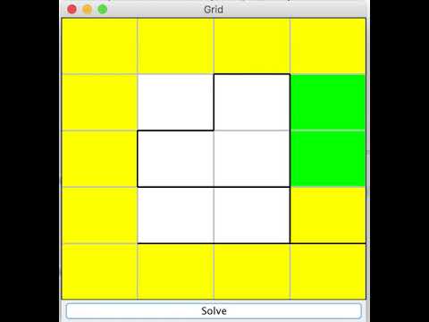
- Note 1: The basic structure of GUI is to use 5 by 4 JPanels, which enable us to assign wall values to each panel according to the input values from the main program and color the edges accordingly.
- Note 2: The GUI program accepts a list of in order of nodes that are visited by the robot, and based on this, color each panel (grid) in sequence to simulate the motion of the robot, which is what the video above is about.
Random Maze Generator
Upon the successful completion of simulation on several mazes, our team was inclined to prematurely conclude that the work on algorithm was done. However, we wanted to test the efficiency and robustness further, in particular with the ‘corner’ cases, in which the mazes are intentionally designed to confuse the robots. So far, due to our inexperience with the testing with physical mazes, we were not ready to artificially come up with good sets of corner cases. In other words, we had to generate as many random mazes as possible and try our algorithm on.
It is easy to draw 5 by 4 arrays on paper. On the contrary, it is very slow and toilsome to convert the walls into binary numbers and hard-type them onto the program. Therefore, we wrote a simple script that randomly generates mazes. We assign the ‘level’ parameter from 0 to 1 that is proportional to the number of walls.
- Note 1: We have to be careful about assigning the wall values to the sides of grids that overlap with each other. After randomly assigning wall values, adjacent sides have to be checked to make sure they have the equal value. Otherwise, the wall half-exists and half-not exits, and the robot is bound to get confused!
- Note 2: The boundary walls should always be added.
- Note 3: This is not the most efficient way to generate a good maze, because the routes can be easily blocked in the vicinity of the starting point, and the bulk of grids are unreachable, especially as we increase the level parameter. We tried to solve this issue by weighting out the random values (larger weight for smaller (x,y) value, so that walls are generally spread out on the farther grids from the starting point). This is not yet the best way to generate a complex, yet logically sound maze; we will work more on the logic of the script to do more complete simulations.
Arduino Language
 The next step is to transfer our codes in Java to Arduino. Our codes in simulation were not directly transferrable to Arduino, and we had to write a new program, albeit with the same logic process. Please refer to our code file on Github repository for details. Several things to point out:
- The grids are in linear array, starting at 0 from top-left corner to 19 at the bottom-right corner, where the robot will start its trip.
- Each grid holds 16 bits information as follows. X-coordinate is 2 bits (from 0 to 3), Y- coordinates 3 bits (from 0 to 4), 4 bits for wall information, 1bit ‘visited’ boolean to mark visited grid, 5 bits of backpointer linear grid number (0 – 19), and lastly 1bit ‘isSpecial’ boolean.

- We initially tried to use bit-shifting on uint16_t variables; however, it seems as though Arduino does NOT support 16-bits bit-shifting, and we had to rely on regular math operations, whenever we had to get a certain information out of 16 bits and change it to a different number whenever necessary.
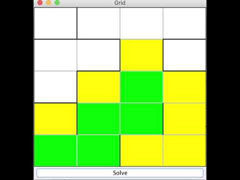
Before we end the section on algorithm, we want to show you one more video of GUI simulation. The unreachable areas (the areas that are completely surrounded by walls) are marked with gray color (then you know the robot finished its exploration!)
In real life:
In order to test our algorithm in real life, we had to create a FSM to control the movements of our robot, shown below:
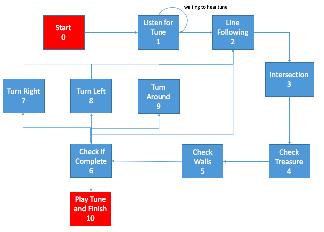
In the competition, the robot will start at State zero, the “start state”, and automatically enter to State One, in which the robot will be waiting for the tone. These two states however are currently bypassed in this Milestone.
For the Milestone, the robot will automatically start in State Two (line following), the robot will start line following immediately after starting. However, in the final, we will start the robot in the intersection state to check for walls immediately after initiating.
State four (check treasure) and state five (check walls) are pretty straightforward. For this Milestone, we did not implement any treasure detection, however, wall detection is implemented to determine what the next block the robot should traverse to. For wall detection, we used the wall detection code written in Milestone 2.
State 6 (Check if Complete) is the state where we will be implementing the search algorithm and determine whether the entire maze has been searched. If more exploration is needed, the search algorithm will determine if the robot needs to turn right, left, or turn around;. This is why this state has five options for the next state.
Once the robot has the correct orientation, provided that the maze has not yet been fully explored, the robot will go back and enter the line following state (state 2) again, starting the entire loop again.
Here is one of the robot’s attempts at travelling through the maze:
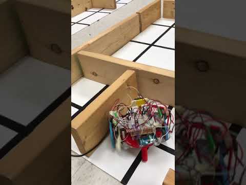
If you have just watched the video, you might be shocked at how bad our robot looks and how its behavior does not seem to make any sense. But in fact, it does not look as bad as it seems.
Firstly, as you will read soon, we are in the process of making a complete overhaul of our original robot design. Because we have been focusing on the redesigning and reshaping parts, our robot has been neglected. The sensor connections are pretty weak and inconsistent with all the lines and connectors flying around each other; the wall sensors are duct-taped and tilted in unpredictable direction, which makes it very hard to set any reasonable wall-threshold value. But again, we plan to redevelope the entire robot this coming week with new chassis and new line sensors. Please bear with us until our robot is reborn with a complete transformation.
But, algorithm-wise, we see some progress. The robot is initialized to start at the bottom-right corner, so it assumes there are walls on its east side. We put it on a very tiny maze, where the north side is blocked with a wall. After seeing the north wall, it makes 180 degree turn and comes back to its original position. Again, the robot’s west side looks empty, but in robot’s perspective, it is always blocked, because is still at the last column, which is covered with walls by default. It does not have anywhere to go, and it finishes the exploration and give us its finish sign with red LEDs.
Earlier before this physical testing, we ran the robot while holding it with our hands and printing out the current location the robot is supposedly going using print statement in serial monitor. We verified that when we do not block the wall sensor, it goes through the grid # 19, 15, 11, 7, 3, and then 2, 1, 0 and so on, at least on the serial monitor, as it should (going up north until it hits the topmost row, where it sees this imaginary wall by our default setting, and turning left and go straight again). We also verified that when we block its sensor by putting a block of wall next to it (while we simulate the intersection point by blocking the line sensor), it turns to 14 from 15. And this video seems to complement our earlier testing to a certain extent. Of course, there’s a long way to go, because backtracking–finding a remote node–uses a different logic process within the code.
Roadblocks
Our largest roadblock for the real life test of our algorithm was the fact that our robot was still missing a lot of features, the most important being wall sensing. We are in the process of redesigning our robot (look at the improvements section for details), but we realized we wouldn’t have time to test the algorithm with the new designed robot before the due date, so we decided to use our original robot.
Improvements for the Future:
In terms of our algorithm, we still need to consider the following:
- Cost factor of turning: The more the robot turns, the more time it will take to finish its maze exploration.
- Information about treasurers: Obviously, we need to find and identify the treasurer frequency.
- General algorithm: There is a lot more room for improvement in backtracking algorithm. We arbitrarily define which grid to look at neighbor nodes for Manhattan distance calculation, and the condition for ‘isSpecial’ has not been studied fully. We are currently looking into an option of employing Breadth First Search (BFS) for backtracking, but in slightly different way to minimize the use of memory as much as possible. Also, whenever we pop a grid from the stack, instead of choosing the topmost one, we can go through all nodes in the stack, find the shortest distance one first, and adjust the order of stack accordingly.
- Systematic simulation: Since we can run our simulation unlimited time using our random maze generator, we can do statistical testing. We plan to add more case-check to make our algorithm more efficient. But, will that be worth it, in spite of more memory usage? Will it actually improve our result in a concrete level, or will the change be so small that we might not use it to lower the level of complexity in our coding to make our debugging process easier? And lastly,
- Contingency: What if the robot runs out of battery? What if it runs out of memory? And what if it loses its main black tape grid and start wonder out to empty grid space? These are not expected to happen with careful preparations, but they still can, and the algorithm should be able to deal with these contingencies. As we test more on the physical robot, we will identify them and make our algorithm more robust by accommodating them into our final code.
Right now, we also have a lot of modifications we want to make to our robot, including the following:
- Changing the structural design of our robot
- Laser cutting a new chassis
- Placing the motors on top of the chassis.
- 3D printing a new ball bearing holder to match the size of our changes
- Printing a PCB
- Implementing a new line sensor
1. New Structural Design:
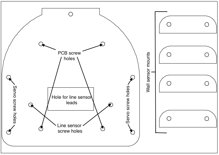
The overall purpose of the new chassis is to make room for the new line sensor and PCB. The wall sensor mounts will also be laser cut and glued directly onto the chassis.
2. Schematic of new PCB:
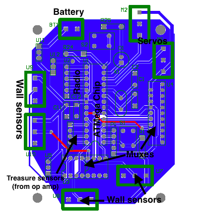
This diagram gives you a general idea of how our PCB will work. Once we mill out our design and test it, we will see what changes need to be made. We might also add an op amp circuit on a separate PCB for our microphone, but that isn’t included in the diagram right now.
3. New Line Sensor:
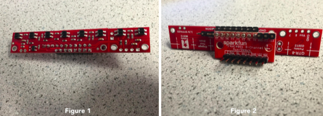
The new line sensor we chose is the Pololu QTR-8A Reflectance Sensor Array. A picture of our sensor can be seen in Figure 1. This line sensor has the following specifications:
- Infrared phototransistor based reflectance sensor array
- 3.3V to 5V operation
- Measures only 2.95” x 0.5” x 0.125” and weighs 3.09 grams
In order to be able to use all 8 of the line sensors, we had to add a mux to it as seen in Figure 2. We soldered the pins of the line sensor to the corresponding pins of the mux. In hindsight this wasn’t the best idea since it eliminated some of our flexibility in how we use the line sensor.
Go To:
Home Page
Milestone 4