The purpose of this lab is to implement grid localization using Bayes Filter. This is the process of determining the position of mobile robot relative to its surroundings. In this lab, we work with the simulation and in Lab 12 it is integrated with the robot.

Discretizing the Environment

The lab space setup which we will eventually test our robot in is a 12ft by 9ft space with obstacles. As the robot can move in two dimensions and rotate as well, the robot pose is three dimensional defined by (x,y,theta), where the first two components specify the x and y position of the robot in the grid and the theta value specifies the rotation. However, as this space is continuous, we need to discretize it for the Bayes theorem.

• x axis: 12 grid cells; each grid cell of size 1 ft (0.3048m) representing [-5.5,+6.5) on the x axis at 1 ft intervals.
• y axis: 9 grid cells; each grid cell of size 1 ft (0.3048m) representing [-4.5,+4.5) on the y axis at 1 ft intervals
• rotation: 20 degree intervals in the range [-180,180) degrees. For example, all rotations in [0,20) degrees will label as a rotation of 10 degrees. Similarly, all rotations in the [340,360) degrees will be labeled as -10 degrees.

Now that the robot’s world space as been discretized, we can use the Bayes Filter to implement grid localization.

What is a Bayes Filter ?

The trajectory plotter below plots (1) Ground Truth in green – where the robot is and (2) Odometry in red – where the robot thinks it is based on sensor reading. Clearly, the odometry is not very reliable and using non-probabilistic methods that only look at the odometry for localization can lead to poor results. We will use a probabilistic approach with the Bayes Filter to determine the pose of the robot for better results.

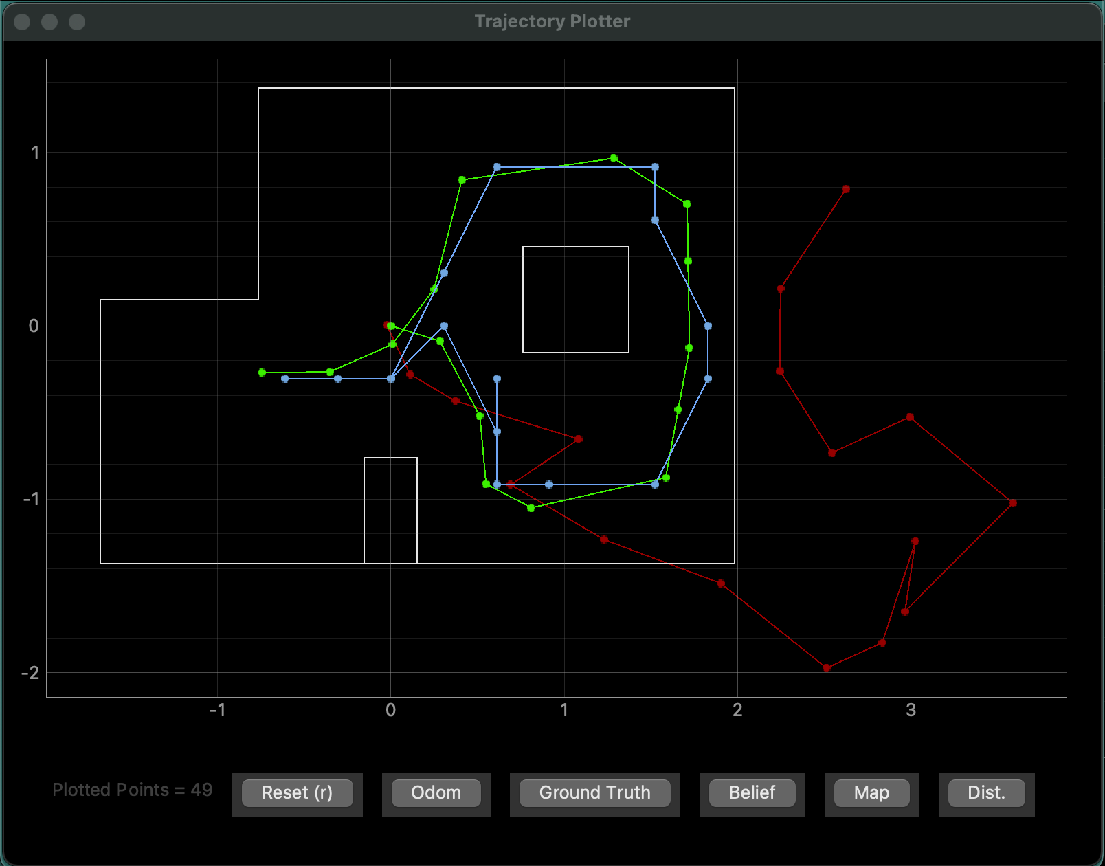
Initially, the Bayes Filter has an initial belief – a belief is a list of the probability that the filter believes it is in a particular pose for each possible pose. Once the robot makes a movement, this belief is updated. The Bayes Filter algorithm in every iteration implements two steps, similar to Kalman Filter used in Lab 7. In the prediction step the control input data (movement command given) is incorporated into the existing belief, creating the prior belief, a new belief based on the control input data and the previous belief. This step adds uncertainty to the belief. Next, sensor measurements are taken, and the update step is performed to incorporate these observations into the prior belief from the prediction step. Clearly, the update step decreases the uncertainty in the belief as the sensor observations are included. The diagram below is a algorithmic representation of Bayes Filter.

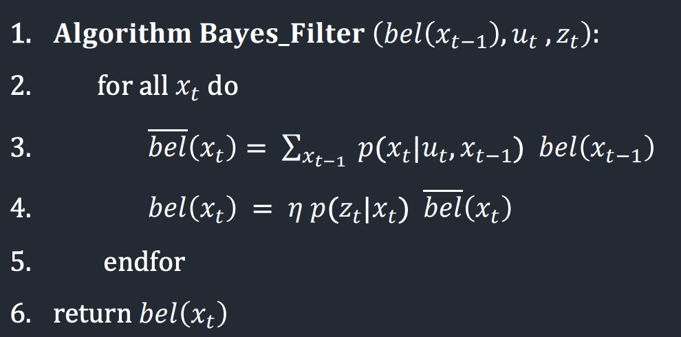
For this lab we were provided with a code skeleton and had to implement the key functions. I first read through the code provided and the lab notebook to understand the code structure. Given Below is the algorithm and use of every function we had to implement.

Gaussian Function

Motion Model

We used an odometry motion model for this lab. Odometry data was recorded before and after the each movement of the robot. We have described a single motion u using three parameters delta_rot_1, delta_trans, delta_rot_2. This can be thought of dividing the motion in to three parts. The first parameter is the amount the robot rotates so it can follow a direct path to reach the new position while moving forward. The second parameter is the translation, it is the distance the robot moves to reach the new position. The third parameter is the amount the robot rotates after reaching the new position to match the current yaw. While completing a trajectory in real life, it does not make sense for the robot to rotate twice once before and once after the forward motion. In the discretized environment model, we need to be able to calculate a movement u between any two states/poses in the grid, which includes the yaw angle. For example, if the robot moves from (0,0,90) to (10,0,90), there is no way to describe the motion in a one rotation and translation parameters.

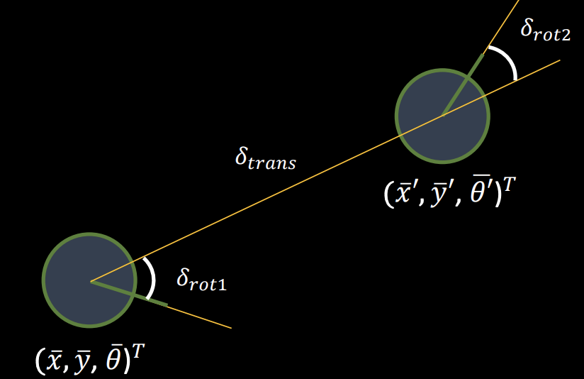
The compute_control function calculates motion/control input given a previous state and current state. The math.dist function is used to calculate the Euclidean distance between the previous and current poses to measure the translation. The rotations are calculated as described in the diagram above. The math.atan2 returns the angle in randians, so the np.rad2deg function is used to convert it to degrees. I have also normalized both the rotations using the mapper.normalize_angles function to ensure that it is the (-180,180) range.

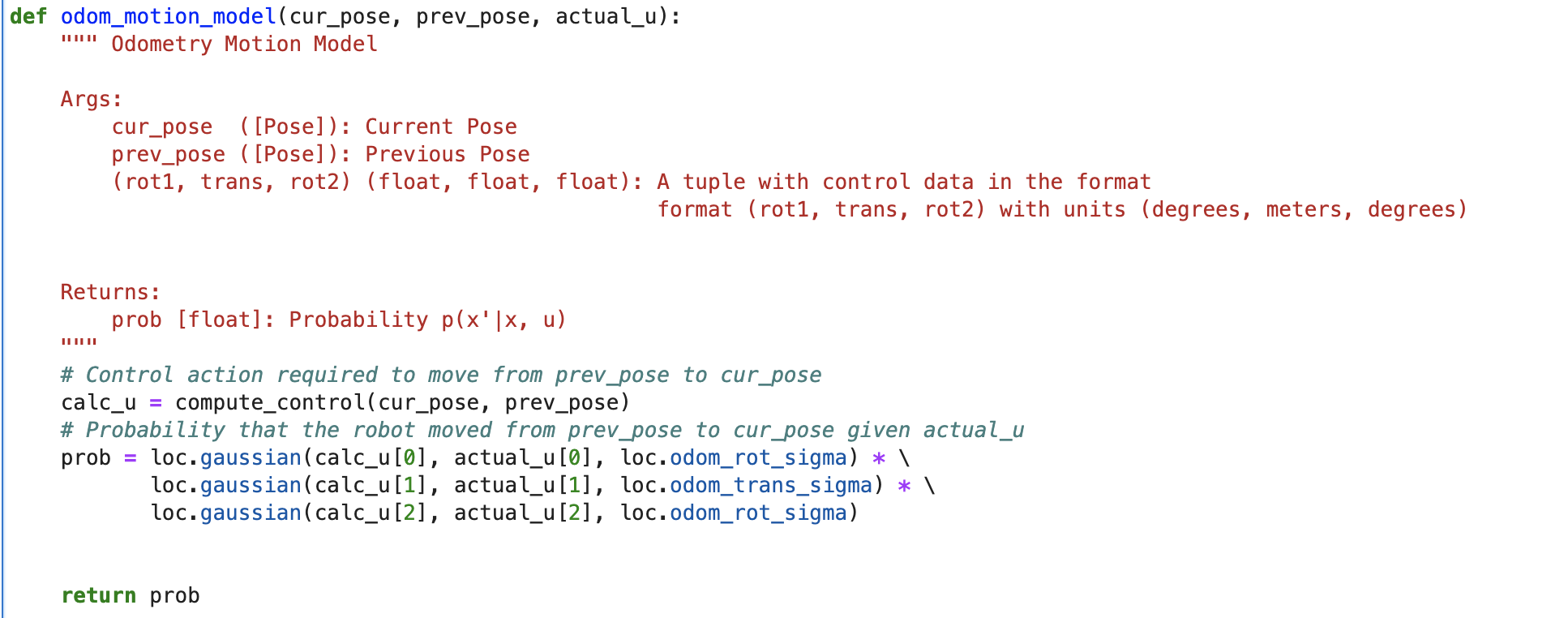
The odom_motion_model function returns Prob(curr_pose|prev_pose,actual_u) , - the probability that robot moved from prev_pose to curr_pose given the control input actual_u. We first calculate calc_u using the compute_control function to find the necessary control action required to move from the provided prev_pose to curr_pose. We use the gaussian distribution to introduce noise and to find the probability that the robot completed the calc_u transition given the actual control action was actual_u. To do so, the loc.gaussian function is applied for each of the three parameters delta_rot_1, delta_trans, delta_rot_2, with the calc_u parameter as the value, actual_u parameter as the mean (this was the actual control input, so it should be the mean of the executed motion) and odom_rot_sigma and odom_trans_sigma as the standard deviation for the rotation and translation respectively for noise. The resultant probability is the product of the gaussian function on all three parameters.

Prediction Step

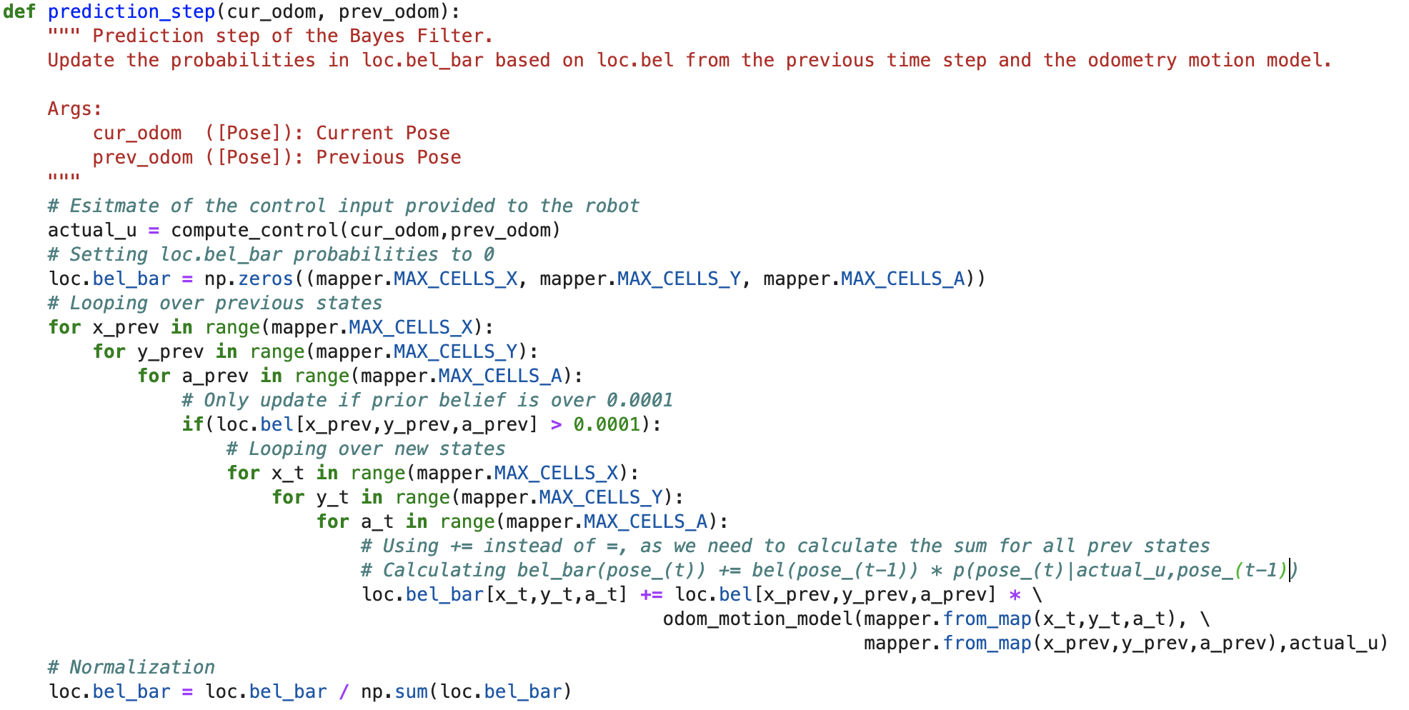
As described before, in the prediction step the Bayes filter predicts the belief bel_bar for the robot’s state based on the prior belief bel and the odometry motion model. The belief probability that robot is in a certain state (x_t,y_t,a_t) is the sum for all possible prev poses (x_prev,y_prev,a_prev) of the product of prior belief that the robot is in state (x_prev,y_prev,a_prev) and the probability that it moved from (x_prev,y_prev,a_prev) to (x_t,y_t,a_t). This is a very heavy computation; So in order to reduce computation time we skipped updating the bel_bar for previous poses with prior belief probability less than 0.0001, as they do not contribute a lot to the belief. Due to this, we first loop over the indices of the previous poses and then the new poses. As we skipped a few poses, we must normalize at the end of the prediction step. We can also skip the normalization here and do it only once at the end of the update state, but since it did not affect computation time much, I kept the statement.

Sensor Model

As mentioned before, the rotation of the robot is discretized into 20 degree intervals. For the sensor model, the ToF sensor is used to record distance measurements rotating the robot at 20 degree intervals starting from 0 degrees, moving anticlockwise up to 340 degrees. An array of 18 ToF sensor measurements taken at [0,20,40,…,340] degrees serves as the sensor observation.

The sensor_model function takes in an array with the true observations for a particular pose in the grid. The true observations for each pose are precached. It calculates the likelihood of each sensor measurements based on the fact the sensor observations recorded after the robot’s most recent movement, which is stored in obs_range_data property of the BaseLocalization class object. Once again, we use the gaussian function to find the likelihood of each sensor measurement, with the true observation as the mean and the sensor_sigma as the standard deviation. The sensor_sigma value is the noise parameter for the sensor model. An array of the calculated likehoods for each of the 18 measurements is returned. Basically this function returns the probability that the collected sensor observation are from a particular pose from where the true observations are provided.

Update Step

Lastly, we need to implement the update step for the Bayes filter to incorporate the sensor measurements into the belief. Similar to the prediction step, this function iterates over all possible poses to update the bel belief got every pose. According to the Bayes Filter algorithm, for each pose the prior belief bel_bar is multiplied by the probability the current sensor measurements are from that pose to update the belief. As we use the sensor_model function to calculate the likelihood for each individual measurement, we take the product of all these probabilities ( AND operation) to get a single probability value. This is done using the np.prod function. Thus, the belief for each pose is updated based on the sensor measurements taken after completing the new movement. Lastly, we normalize the belief matrix to ensure that the probabilities add up to 1. I did not add a conditional statement like in the prediction step, because the operation to update each belief is quick and there are no more iterations after the first three loops unlike the prediction step.

Results

Given below is a video showing the simulation and the plotter implementing a trajectory path. The Bayes Filter belief is plotted in blue, the odometry in red and the ground truth in green. Notice that the belief follows the general path of the ground truth, and is way better than the odometry.

To experiment, I tried to change the noise parameters for the odometry and sensor model in the config folder. The noise currently used for the sensor model is 0.1, which is about 1000 mm. In my opinion, this is a lot, but considering how noisy the ToF sensor data is and the fact that our observations may not be exactly at 0,20,40 … rotations, it makes sense. I tried changing this to 0.5 and 0.2.

On analysing the belief probability, for each of the points, I noticed that the belief probability after the prediction step is usually low in the 0.1-0.2 range. Whereas the belief probability after the update step for the estimated position is extremely high, almost 1.0 for some parts. In cases where the estimate is wrong, the probability is lesser, around 0.6.

Notes

While we wrote our own code, I discussed my ideas with Krithik Ranjan.

[Submission Note] Code and video has been uploaded at 2:30 pm on 26 April, this can be verified on github.