In this lab, we used the Bayes filter implemented in Lab 11 and perform localization in the lab environment setup. It was interesting to see the performance of Bayes filter-based localiztion which we had tested on the simulator, in real life. The tasks for this lab, involved running the update step of the Bayes filter in four different positions in the lab environment and discussing the results.

I collaborated with Krithik Ranjan (kr397) and Aparajito Saha (as2537) for the this lab. We used Krithik's robot, as it had the best PID control for 20 degrees rotation from Lab 9. We used Apu and my laptop to connect to the robot via Jupyter notebooks. Collaborating with others helped me with lab and interpreting the results better as we could bounce ideas off of each other.

Localization Module in Simulator

We were provided with a fully functional optimized Bayes filter implementation as a part of the Localization class that works on the virtual robot, along with two notebooks - lab12_sim.ipynb that demonstrates the Bayes filter for the virtual robot and lab12_real.ipynb that gives a skeleton code for the real robot. First of all, I compared my code from Lab 11 to the provided Localization class. The functions used for the predict step were very similar. However, for the update step the code was more efficient compared to my solution. It used numpy processing instead of the extra helper function and function like deepcopy instead of extra loop to iterate over the beleif arrays. The solution also precached the views (the ray casting values for every position) before starting the Bayes Filter.

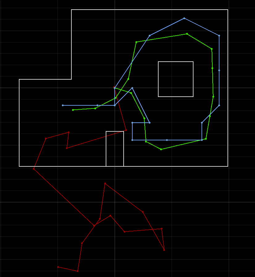
We ran the lab12_sim.ipynb Jupyter notebook to see the implementation of the Bayes Filter based Localization on the simulated robot. The robot performs the trajectory shown below by localizing at every point in the trajectory. The plot below shows the simulated run of the robot - the green line represents the ground truth, the actual position of the robot; the red line represents the perception of the robot based on the sensor readings, this is its odometry; the blue line represents the beleif of the robot after localizing (predict and update step) at each point. As seen in Lab 11, the belief is close to the ground truth. We used the print_prediction_stats and print_update_stats functions of the Localization class to look at the beleifs at each step and the probability of that particular pose.

Localization on the Robot

Next, we had to complete the skeleton code provided in lab12_real.ipynb notebook to implement localization on the robot. We were provided with a RealRobot wrapper class skeleton which is used by the Localization class to communicate with the robot. For this lab, we had to implement the perform_observation_loop member function to get the ToF sensor data readings and store them in the obs_range_data member variable.

Observation Loop

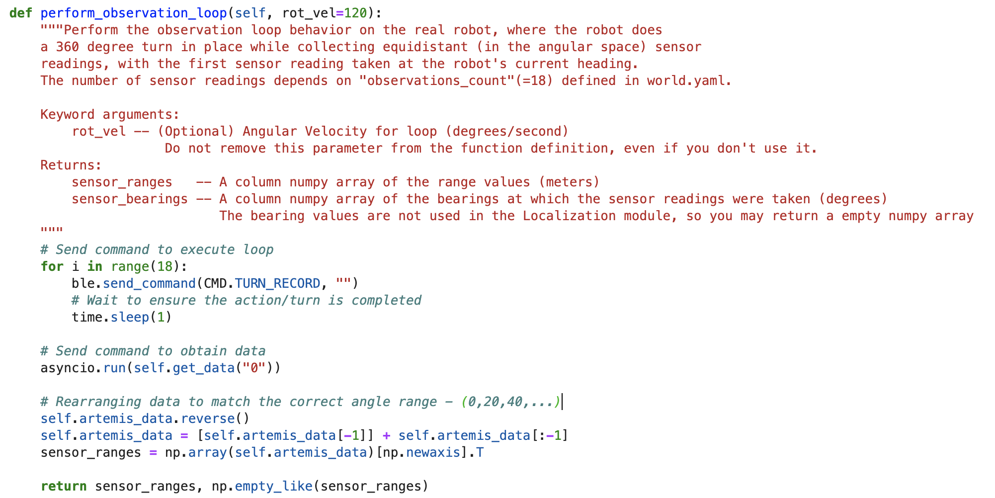
The robot's rotation is discretized into 20 degree increments, so each observation loop involves recording the ToF sensor's data measured at 18 angular positions in 20 degree increments ( +0, +20, +40, ..., +340). The positive angles are along the counter-clockwise direction. To implement an observation loop, the computer sends the robot the TURN_RECORD command 18 times. Each time the command is sent, the robot records and stores the ToF sensor data at current position and then turns 20 degrees (tuned angle). This is similar to the code used in Lab 9. After completion of the all the movements, the data collected by the robot at each position can be retrieved by sending the GET_DATA command. The PID rotation in the robot was set up and tuned to rotate in clockwise direction (with ToF placed in the front). As the PID tuning worked perfectly for 20 degree rotations, we decided to reuse the code instead of retuning the PID in the opposite direction. This meant that the data collected will be at ( +0, +340, ...., +40, +20) degrees. To ensure that the obs_range_data matched the angular positions described before, we had to rearrange the data by reversing the data list but keeping the first value in place (this is for 0 degrees). This can be seen in the code below

Bluetooth Communication

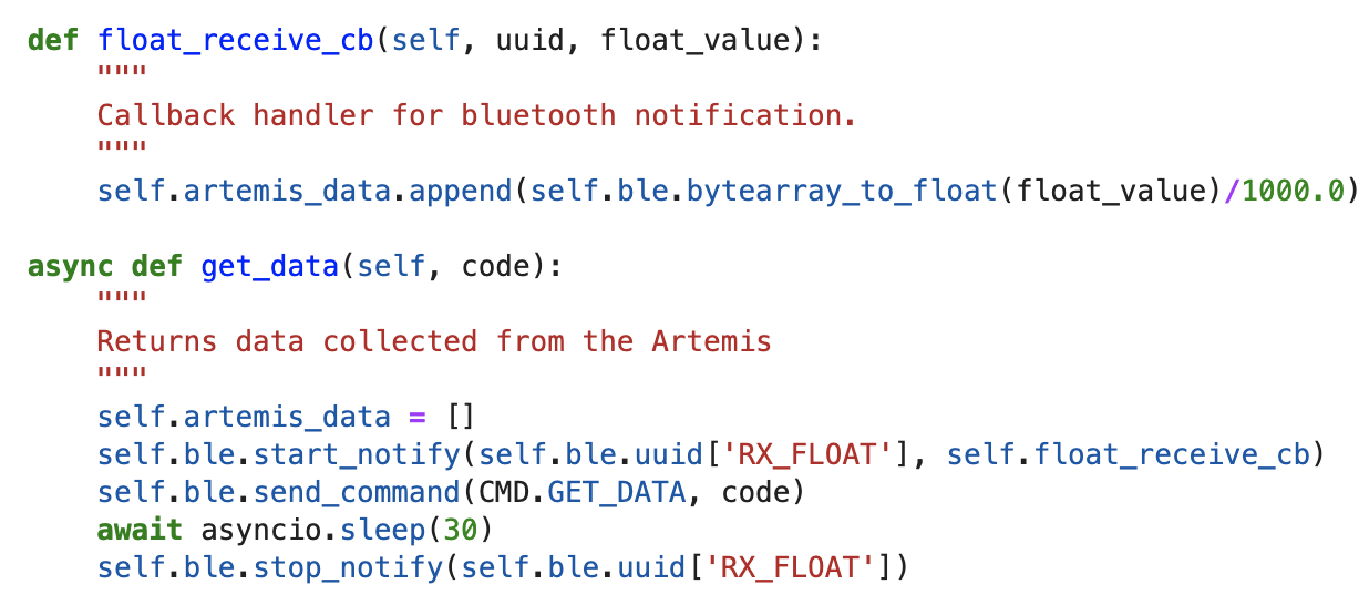
To collect the data from the robot, we used the GET_DATA command, after the observation loop was completed. In all the previous labs, we used start_notify and a callback handler function to recieve data from the robot via bluetooth. We defined the get_data function which first starts the bluetooth notifications, sends the GET_DATA command, waits for 10 seconds to ensure that all the data has been sent over and then stops the notification handler. As suggested, we used await asyncio.sleep to wait for the data. Due to this, we had to add async keyword to the function definition and used asyncio.run to call the function inside perform_observation_loop.

Note that starting and stopping the notfication handler with the function every time does reduce the point of using the notification handler. As our bluetooth connection is finiky, we used this method. We could have also integrated the bluetooth by polling for the readings after each turn command and the robot sending the ToF sensor values as and when it measures. However, this would involve waiting in between turns until the sensor data has been sent. This would mean that we will have to add the async keyword to the function definition of perform_observation_loop and get_observation_data.

Testing

Now that we had implemented the Bayes filter localization, we implemented our task of performing the update step at five of the markered positions (we also included the origin) and get the belief at each position. Before running each step, we re-initialized the grid beliefs, so that the robot has the same initial beleif for all positions. In the update step, the robot first gets the obersvation data at the current position, and then uses the pre-cached views and the current belief matrix to calculate the probability that the robot is at a particular pose for every possible pose. The pose with the highest probability is considered as the estimated pose. Note that as in the previous lab, each pose is represented as (x, y, θ), where x, y are the position of the robot in the grid and θ is the rotation of the robot with respect to the positive x axis. Due to discretization, the rotation θ is in incremenets of 20 degrees (-170 -10, .. 10, 30, ..., 170). For example, if the robot has a rotation in the range [0,20), θ will have a value of 10. Similarly, the x, y coordinates are also discretized into a 12 by 9 grid, where each cell is 1 ft or 0.3048 meters.

Results

We ran the update step at the following five positions, three times each - (0,0), (0,3), (5,3), (5,-3), (-3,-2). The robot was always placed with the ToF sensor towards the right (0 degree rotation). Below, we have provided the data collected at each position, the Bayes Filter estimate and probability at the estimated pose for best of the three runs.

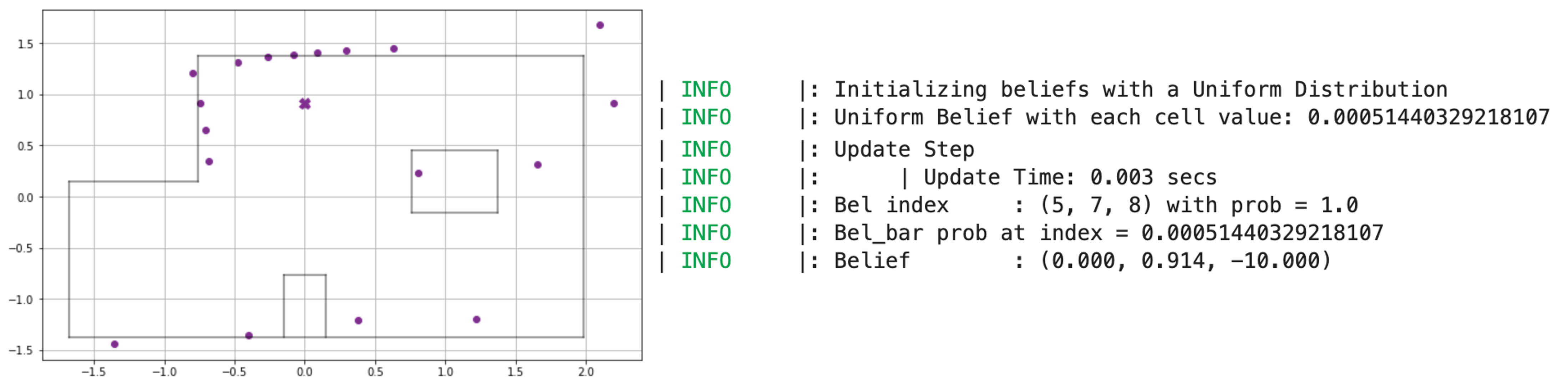
1. Point 1 - (0,0)

   

2. Point 2 - (-3,-2)

   

3. Point 3 - (0,3)

   

4. Point 4 - (5,-3)

   

5. Point 5 - (5,3)

   

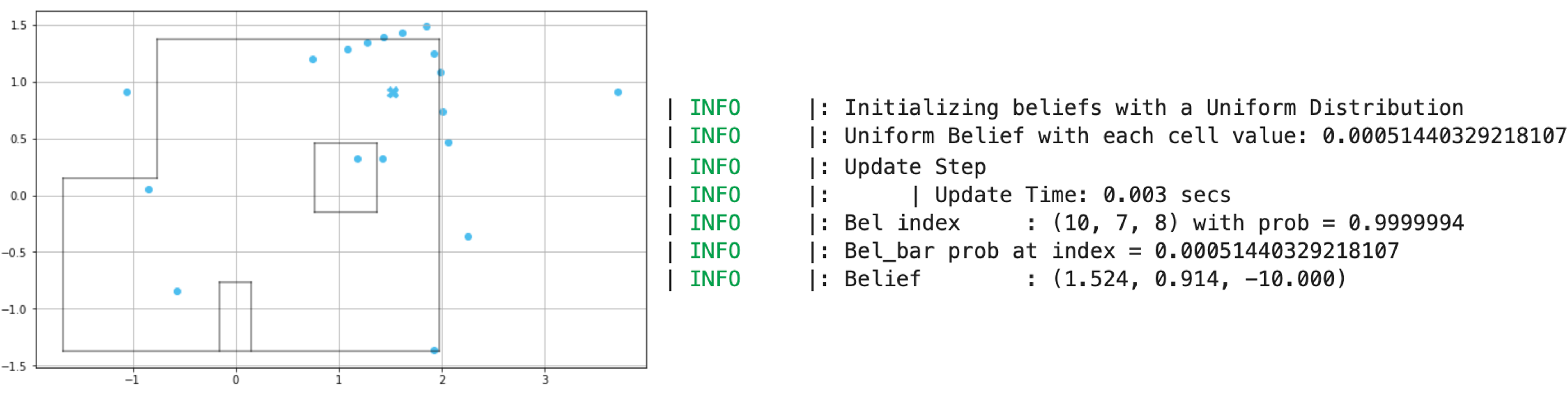
Surprisingly, the robot was able to correctly localize at all five position markers. While the ToF sensor readings for long distances were quite inaccurate at certain points, especially from (0,0), the robot was able to localize correctly. Even the probability at the estimated pose was very high in each case (0.99 or 1.0). It amazed me that the robot probability was so high, considering we had only run a single step. The rotation angle estimated by the robot in each case is -10 degrees, where as per the discretization it should have been 10 degrees as the robot was kept at a 0 degree rotation. We could account for this slight error due to the drift while doing 20 degree turns 18 times, so the readings might be slightly more towards the right than it should have been as the robot moves clockwise.

We did face some issues while localizing at (5,-3) point. While at other markers the robot always localized correctly, the robot did give some wrong readings at this position. Some times the robot estimated that it was at (3,-4, -50). Below are the ToF sensor readings and the output values of when the robot localized incorrectly. A point to note is that the belief probability is 0.88, which is significantly lesser than the belief probability when the robot localizes correctly. In this case, we also checked for the next highest belief probability which was for the (5,-3). It was interesting that when the robot estimated incorrectly at this position, it always estimated it be at the same (3,-4) point. We could not understand why it estimated it to (3,-4) as the surroundings of both the points are very different. However, if you consider the robot taking clockwise readings at position (5,-3) starting at 0 degrees, they could be similar to what the robot would observe at position (3,-4) starting at -70 position. This error could also be because the robot is in a corner has similar observations to other positions in the grid.

Conclusion

I am quite happy with the results from this lab and excited to use localization for path planning in the next lab. I am hopeful that we should be able to correctly localize the position (x,y coordinates) for the next lab, but I am not sure if the estimated rotation angles will be accurate. Thank you to the course staff for helping me understand this lab, especially Vivek for helping understand the code and bluetooth and Jade for interpreting the results