Investigating Anemia Levels in Women

Report

Introduction

Anemia is a primary contributor to the global health burden, being the most common blood condition worldwide. Low numbers of red blood cells associated with this condition can impede the body’s ability to perform physiological functions and increase the risk of mortality.

Our project centers on two analyses. Our first analysis aims to answer our research question on whether women from developing countries have higher rates of anemia than those from developed countries. The variables we will be using are country classification (country_classification, i.e., whether the country is developing or developed, and mean hemoglobin levels (mean). Our second analysis focuses on how pregnancy status affects anemia rates in women and the relationship between the pregnancy variable and the mean hemoglobin levels.We will analyze the relationship using the mean and pregnancy variables within the dataset.

Main findings include that there is a significant difference between mean hemoglobin levels for women between developed and developing countries, as well as a significant difference between mean hemoglobin levels for pregnant and non-pregnant women. Outlining these distributions can bring light to what appropriate scales and target areas of prevention measures can be taken against anemia for vulnerable populations.

Data Description

The original dataset from which our dataset was derived was funded by the World Health Organization and created for the analysis of hemoglobin data for global anemia estimates in 2021. Original data was collected via health and nutrition examinations, as well as household surveys, and anonymized individual records drawn from various databases. Each observation in this original dataset appears to group a specific sample of individuals, based on country, year the data was collected, their sex, age range, and pregnancy status, with sample size, mean hemoglobin levels, percent of individuals in the sample falling within specific hemoglobin level thresholds, and the organization through which the survey was administered recorded.

Specifically, we narrow our analyses to 2 questions – that is, the relationship between estimated mean global hemoglobin levels (mean) in women based on country status ((country_classification), developing/developed), and the relationship between estimated mean hemoglobin levels (mean) in women based on pregnancy status ((pregnancy) pregnant/non-pregnant). Observations in the former include data values for individual countries and attributes include mean hemoglobin levels and country classification. Observations in the latter include data values based on individual samples of women from the dataset, and attributes include mean demoglobin levels and pregnancy status.

Additional preprocessing of the original dataset into our current dataset to be specifically integrated into our two research analyses include filtering for sex (samples with women only, mixed sex samples were excluded from the data), and mutating the dataset to include an additional column for country_classification labeling countries by status (developed or developing) based on the list of developing countries as declared by the Minister for Foreign Affairs. More information on data preprocessing can be viewed in the appendices.

Primary limitations of our dataset include unequal distribution of sample data – e.g., that the number of sample categories for different countries differ. This may result in skewed or decreased accuracy of representations of population data. In an effort to address this limitation in our study, we intend to perform additional preprocessing of data by filtering out specific data for uniformity of our dataset.

Data Analysis

First Analysis - Do women from developing countries have higher rates of anemia than women in developed countries?

Our first analysis investigates the relationship between country classification as our explanatory variable and mean hemoglobin levels of women as our response variable. The variables we use to analyze the relationship primarily involve country classification (country_classification, i.e. whether the country is developing or developed) and mean hemoglobin levels (mean). The following considerations were made in the investigation of this question:

First, we read the excel file and cleaned and tidied our data through the use of the select() and filter() functions so that our dataset contains clean and useful values in the context of our first research question.

# A tibble: 2 × 2
  country_classification mean_hemoglobin
  <chr>                            <dbl>
1 Developed                         127.
2 Developing                        119.

Next, as the variables we are investigating are binary categorical (country_classification) and continuous numerical (mean), we then visualize the analysis using a horizontal bar plot showing the relationship between mean hemoglobin levels and the country classification. A look at all relevant countries shows generally that developed countries have higher hemoglobin levels compared to developing countries.

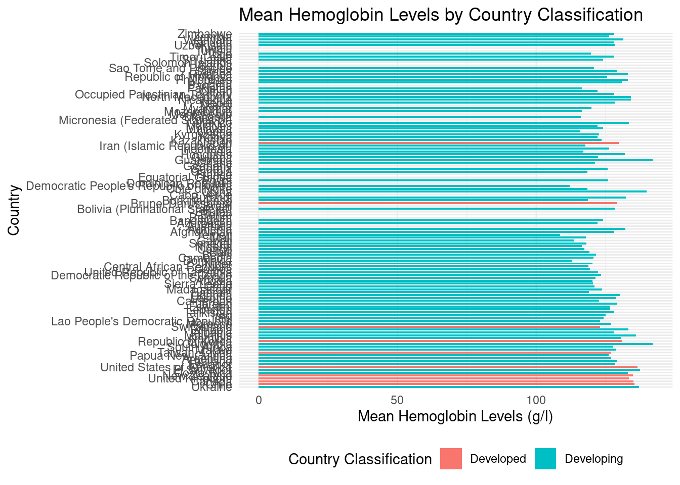
Grouping each country classification together, we create a more direct comparison of developed and developing countries’ mean hemoglobin levels; it appears indeed as if mean hemoglobin levels are higher for developed countries as compared to developing countries. Further steps to analyze this possible relationship are addressed in Evaluation of Significance and Interpretations and Conclusions.

Second Analysis - How is pregnancy related to anemia is women?

Our second analysis investigates the relationship between pregnancy status as an explanatory variable and anemia rates in women as our response variable. The variables we use to analyze the relationship primarily involve pregnancy status (pregnancy) and mean hemoglobin levels (mean).

Similarly to the first analysis, we first cleaned and tided our data through the use of select() and filter() so that our data contains clean and useful values to our second research question.

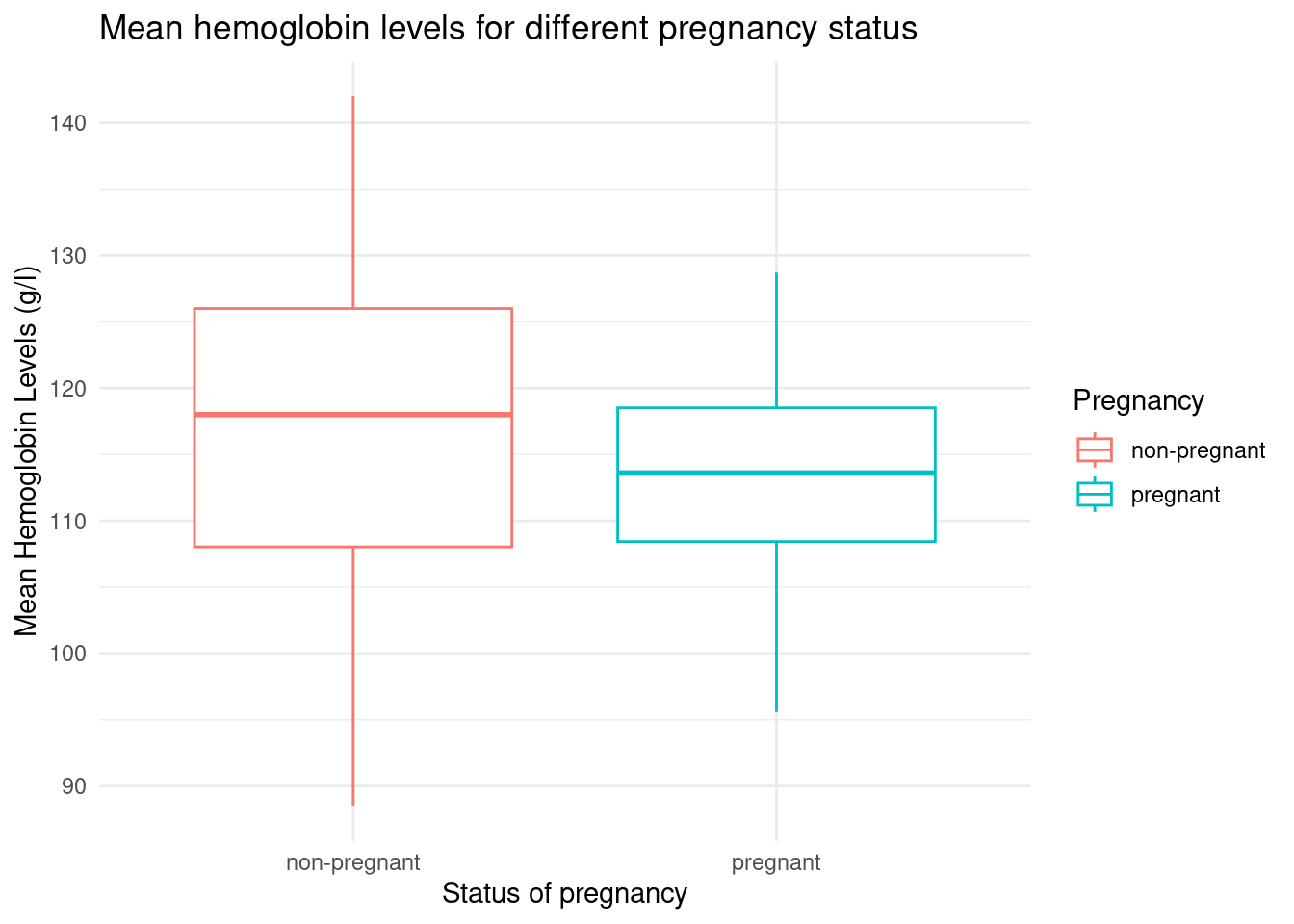
As the variables we are investigating are binary categorical (pregnancy) and continuous numerical (mean), we chose to visualize our second analysis using side-by-side boxplots with a graph of the means and the 95% confidence interval for the mean. This creates a better visualization of the skewness of the data. Furthermore, we decided on ranges and separated the individual means into different ranges.

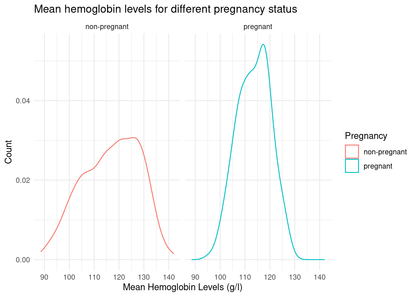
Afterwards, we employed a density chart visualization to show the distribution of the data for both the pregnant and nonpregnant status, facet wrapping for easier comparison.

Additional tidying of data in this analysis included summarizing pregnancy status and mean hemoglobin values and summarizing hemoglobin values and the country classification. In other words, we explore the use of descriptive statistics (mean, maximum, minimum, etc.) to help summarize our data, which we implement into a summary of its linear regression model in the following section.

Evaluation of significance

We also use a hypothesis test to help give an input on the statistics that we have observed. Data and results will be reported and any specific limitations will be mentioned.

First Analysis

Hypotheses
- Null Hypothesis: There is no difference between mean hemoglobin levels of women in developing countries compared to mean hemoglobin levels of women in developed countries (mean hemoglobin levels of women in developing countries = mean hemoglobin levels of women in developed countries)
  \(H_0 = m_{developing} - m_{developed} = 0\)
- Alternative Hypothesis: There is a difference between mean hemoglobin levels of women in developing countries compared to mean hemoglobin levels of women in developed countries (mean hemoglobin levels of women in developing countries ≠ mean hemoglobin levels of women in developed countries)
  \(H_A = m_{developing}-m_{developed} \neq 0\)
  - Or: mean hemoglobin levels of women in developing countries are lower (<) than mean hemoglobin levels of women in developed countries
    
    \(H_{or} = m_{developing} < m_{developed}\)
We use a significance level of 0.5 and a confidence interval of 95%.

                        Df Sum Sq Mean Sq F value Pr(>F)    
country_classification   1   4968    4968   74.65 <2e-16 ***
Residuals              505  33610      67                   
---
Signif. codes:  0 '***' 0.001 '**' 0.01 '*' 0.05 '.' 0.1 ' ' 1
167 observations deleted due to missingness

In terms of analysis, we use an ANOVA test because we have a categorical variable with different groups (different countries) as our explanatory variable and we want to determine whether this measurement differs between groups.

# A tibble: 2 × 2
  country_classification  mean
  <chr>                  <dbl>
1 Developed               127.
2 Developing              119.

# A tibble: 1 × 2
  lower_ci upper_ci
     <dbl>    <dbl>
1     5.94     13.2

# A tibble: 1 × 1
  p_value
    <dbl>
1       0

Second Analysis

Hypotheses:
- Null Hypothesis: There is no difference between mean hemoglobin levels between pregnant women and non-pregnant women.
  
  \(H_0 = m_{pregnant} - m_{non-pregnant} = 0\)
- Alternative Hypothesis: There is a difference between mean hemoglobin levels between pregnant women and non-pregnant women.
  
  \(H_a = m_{pregnant} - m_{non-pregnant} \neq 0\)
We use a significance level of 0.5 and a confidence interval of 95%.
In terms of analysis, we use a linear regression model since the dependent variable is a continuous variable.


Call:
lm(formula = mean ~ pregnancy, data = anemia_data)

Residuals:
     Min       1Q   Median       3Q      Max 
-28.3008  -6.8202   0.6433   7.4106  25.1798 

Coefficients:
                      Estimate Std. Error t value Pr(>|t|)    
(Intercept)            126.357      1.702  74.261  < 2e-16 ***
pregnancynon-pregnant   -9.537      1.756  -5.431 7.47e-08 ***
pregnancypregnant      -12.767      1.835  -6.958 7.26e-12 ***
---
Signif. codes:  0 '***' 0.001 '**' 0.01 '*' 0.05 '.' 0.1 ' ' 1

Residual standard error: 10.07 on 786 degrees of freedom
  (278 observations deleted due to missingness)
Multiple R-squared:  0.06197,   Adjusted R-squared:  0.05959 
F-statistic: 25.97 on 2 and 786 DF,  p-value: 1.203e-11

# A tibble: 2 × 2
  pregnancy     mean
  <chr>        <dbl>
1 non-pregnant  126.
2 pregnant      114.

parsnip model object


Call:
stats::lm(formula = mean ~ pregnancy, data = data)

Coefficients:
      (Intercept)  pregnancypregnant  
           125.63             -12.04

# A tibble: 1 × 2
  lower_ci upper_ci
     <dbl>    <dbl>
1     10.8     13.2

# A tibble: 1 × 1
  p_value
    <dbl>
1       0

Interpretation and conclusions

First Analysis

Based on the ANOVA test, the Pr(>F) value or the p-value for F-statistics is <2e-16. Given that this value is less than our alpha level threshold of 0.05, we reject the null hypothesis that there is no difference in mean hemoglobin levels between pregnant women and non-pregnant women.

Moreover, based on the output of get_p_value(), the p-value is 0, indicating strong evidence against the null hypothesis and in favor of the alternative hypothesis that there is a difference between mean hemoglobin levels for women between developed and developing countries.

Using a 95% confidence interval, we are 95% confident that the true mean hemoglobin level of women in developed countries is 6.086151 to 12.99662 g/l higher than the true mean hemoglobin level of women in developing countries.

Results could be directed to inform scale and focus of measures for targeting interventions to anemia, and lead to important implications for public health policies and interventions for these regions. This conclusion could also prompt further questions or investigations into whether the differences may be a result of disparities accessibility to factors affecting hemoglobin levels such as nutrition, healthcare, etc., or those besides external resources such as genetics or lifestyle; further investigation could in turn help to identify and address these factors in order to improve health outcomes in terms of anemia rates.

Second Analysis

The intercept term is 126.36, which estimates the mean hemoglobin level for the pregnant group.

The coefficient for the non-pregnant group is -9.54 g/L, which means that the mean hemoglobin level for non-pregnant women is estimated to be 9.54 g/L lower than that of pregnant women.

The coefficient for the pregnant group is -12.77 g/L, which means that the mean hemoglobin level for pregnant women is estimated to be 12.77 g/L lower than the reference group.

Both coefficients have statistically significant p-values (less than 0.05), indicating that there is a significant difference in mean hemoglobin levels between pregnant and non-pregnant women. Therefore, we reject the null hypothesis as there is a statistically significant difference in mean hemoglobin levels between pregnant and non-pregnant women.

Using a 95% confidence interval, we are 95% confident that the true mean hemoglobin level of non-pregnant women is 13.24097 to 10.84935 g/l higher than the true mean hemoglobin level of pregnant women.

Results indicate the possibility for a higher risk of anemia in pregnant women. Conclusions from this analysis could be used to inform how interventions and programs may be designed to effectively identify and respond to anemia diagnoses in pregnant women to improve maternal and fetal outcomes. These conclusions can have important implications for the health and well-being of women during pregnancy.

Limitations

There may be confounding variables as there are other factors that would affect anemia rates or hemoglobin levels, such as genetics, medical conditions, dietary restrictions, and other variables. Additionally, the data may not be representative of the population of women in developed and developing countries as the sample may be biased towards specific regions or demographics. As such, while we can infer correlation through the patterns extracted in our data analysis, it may be inaccurate to claim causality between the variables.

Acknowledgments

We would like to acknowledge Dr. Benjamin Soltoff, our course lecturer for his incredible knowledge and aid throughout the process of the project. We would also like to thank the undergraduate and graduate TAs for their knowledge, patience, and help. Lastly, we remain grateful for the surreal amount of resources that are available to us, whether that be from our peers or online resources such as Stack Overflow. Through the use of many great resources and help, we were able to successfully complete our project and ease the transition between each parts.