Where does it pay to attend college?
Report
Introduction
Our main research questions are: How does the classification of a U.S. college affect the starting and mid-career earnings of graduates from that college? Does this vary across different regions of the U.S.? To answer this, we will examine data on the median salaries throughout the career of graduates from colleges from different regions and types. We are interested in researching if there is a significant difference in salary outcomes based on the location and type of college people graduate from. Our analysis will show there is statistical evidence of a relation between a graduate’s starting salary and region of their college.
Data description
We used two datasets that were published on the Wall Street Journal obtained by Payscale, Inc. For salaries_region, each row is a different college. The columns represent the name of the school, the region the school is located in (California, Western, Midwestern, Southern, Northeastern), the starting and mid-career median salaries, and the 10th, 25th, 75th, and 90th percentile mid-career salaries. salaries_type, has the same columns, except the region is replaced with the type of school (Engineering, Liberal Arts, Party, Ivy League, State). This dataset was created and funded by Payscale, Inc. to learn about differences between graduates from schools in different regions of the US and whether the type of school it was had an impact on their financial outcomes. The process in data recording could have been impacted because data from schools with a small graduate class may not be an accurate representation of the entire class, depending on the sample size.
For pre-processing the data, we created two summary datasets for salaries_type_summary and salaries_region_summary, to make it easier to draw conclusions and visualize the data to start of. For all the non-N/A median salaries, we converted the values to numeric. Next, we grouped by type of school/region in the US respectively and created a summary row with a row for each type of school/region, with each column containing the mean of the median salaries at each career stage. For the school type summary, we pivoted the table, so each row represents the mean of the median salaries for all values with the same type of school and career stage. For the region summary, we did the same, except each row represents the mean of the median salaries for values with the schools in the same region and career stage. Finally, we created a merged data set called salaries_joined containing a full_join of salaries_type and salaries_region, meaning that it has a row representing every school from both sets, providing N/As in columns where data isn’t complete.
Data analysis
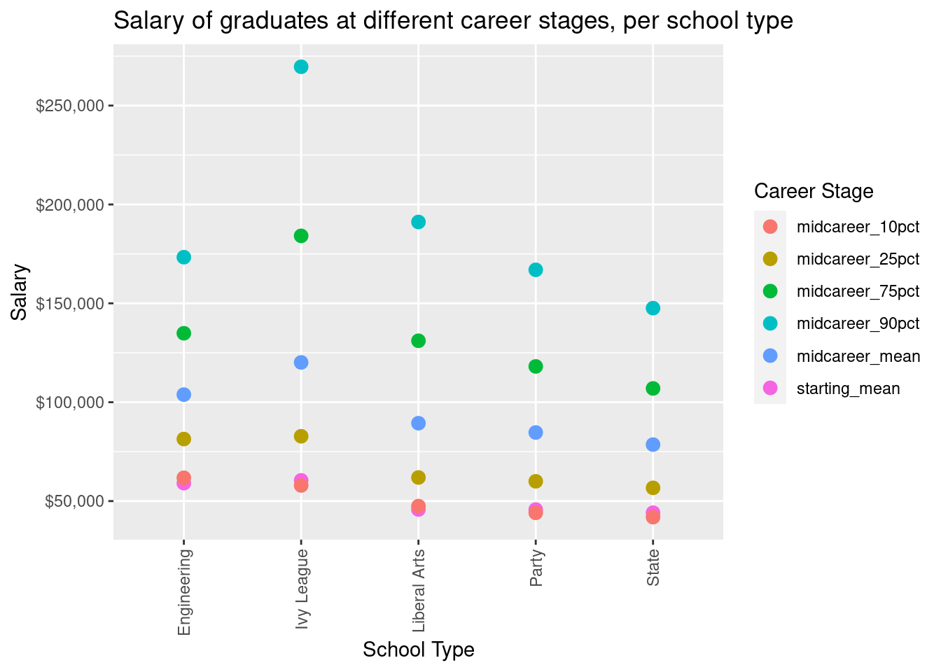
The first plot shows the relationship between the mean aggregate salary of graduates at different colleges and the type of college. The type of schools used for our analysis are state schools, party schools, liberal arts colleges, engineering universities, and ivy league institutions. We used a scatter plot to visualize this relationship, with each point within the same category representing a different percentile within the students who have graduated from a school of the corresponding type. By analyzing this scatter plot we can conclude that all types of schools except Ivy League schools show a similar range of salary percentiles for their graduates. Besides the ranges of these schools being very similar, we can also see they have similar starting mean salaries, with the starting mean salary for engineering graduates being a little higher than the other three types of schools. The range between percentile regions these four types of schools display is very similar. However, our scatter plot does show that graduates from engineering and liberal arts schools have a slightly higher mid-career median salary in comparison to state or party schools on the high percentiles. Ivy League schools show the largest range in salary, with the mid-career top percentiles being the highest salaries by a significant amount. The starting mean salary is similar to that of engineering schools, but the range within percentile regions is still larger than that for other types of schools, setting Ivy League schools apart.
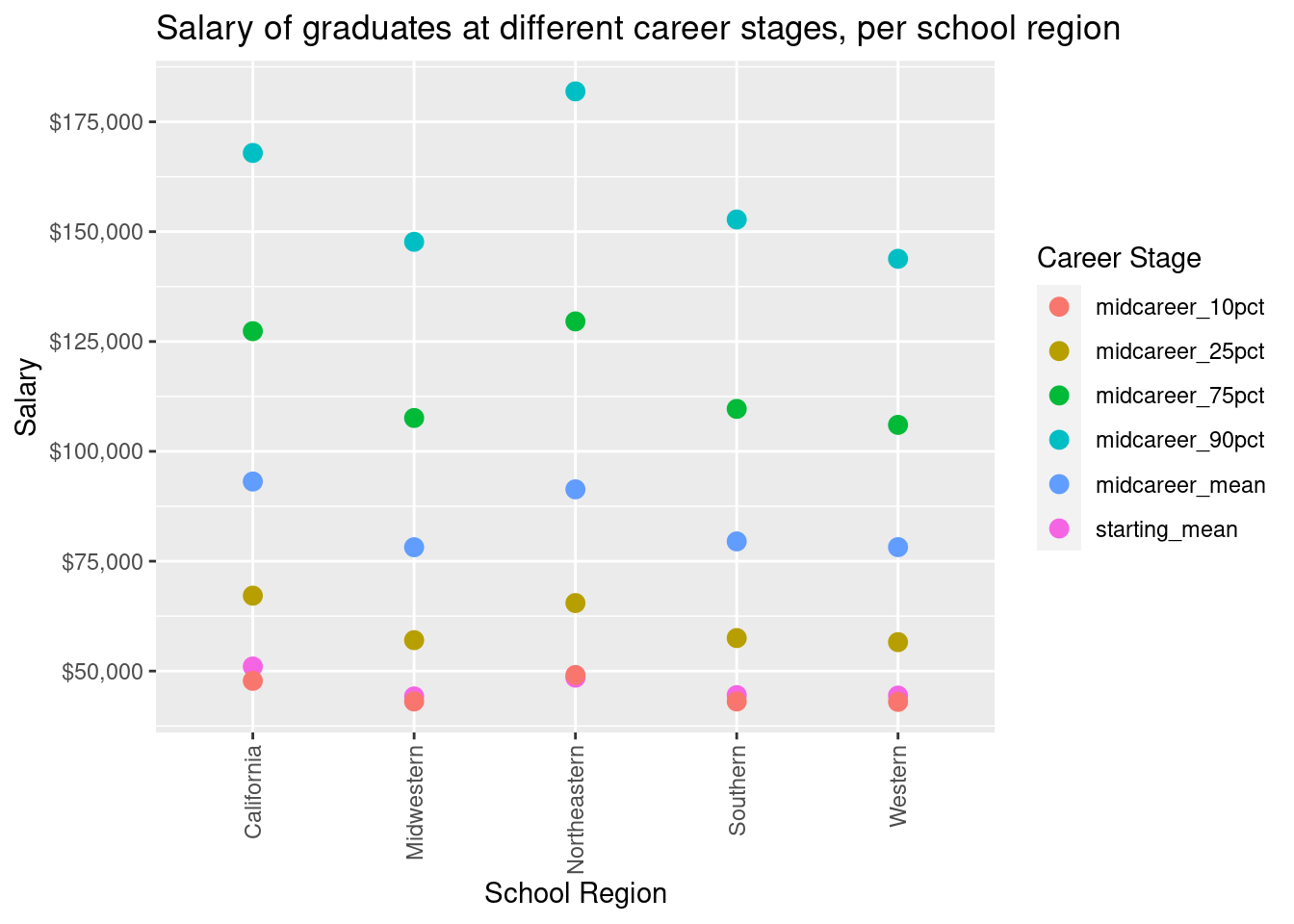
This plot shows the mean of the aggregate salary measures at each college (median starting salary and 10th/25th/50th/75th/90th percentile mid-career salary) within each region. The different school regions used for our analysis are Northeast, South, Midwest, West, and California. We decided to visualize this relationship using a scatter plot. Each color of point within the same category represents a different percentile within the schools falling into the corresponding region. All school regions show similar starting mean salaries for their students. However, the range of salaries and the top of percentiles for graduates do vary among substantially among schools from different regions. Interestingly, these differences in range are a magnification of the slight differences we saw in mean starting salary, but these differences are much more pronounced now. For instance, Western and Midwestern colleges appear to be the colleges with the lowest mean starting salary by a tiny margin; however, they are the two school regions with the smallest range of salaries as well as with the lowest mid-career top-percentile salaries. By the same token, Northeastern colleges are the ones with the highest mean starting salary by a slight margin. The range of mean salaries and mid-career top-percentile salaries followed the same pattern, as Northeastern colleges are at the top of all school regions as these differences were magnified.
Evaluation of significance
College Location vs. Differences in Salaries
Our first analysis intends to identify if there is a difference in the starting salary and mid-career salary for different regions. This could be analyzed using a hypothesis test where we try to identify if the salaries differ in the different regions across the USA. Since there are more than 2 regions, (there’s 5; California, Northeastern, Midwestern, Southern and Western), a simple hypothesis test would not work unless all possible combinations where compared to one another. A better test to understand if there is a difference in the salaries across regions would be to use test of Analysis of Variance, also called an ANOVA test. ANOVA tests whether there is a difference on the means of some quantitative variable, in this case starting salary or mid-career salary, at different levels, or in this case Regions.
The null and alternative Hypothesis will be:
\[ H_0: \text{There is no difference in mean starting or mid-career salary across different regions.} \] \[ H_A: \text{There is a difference in mean starting or mid-career salary across different regions.} \]
If there is enough statistical evidence to reject \(H_o\) at \(⍺ = 0.05\), then we need to find what regions have a difference in mean salaries. We shall do this by comparing Regions to each other.
First we tried to assess if there is a relationship between median mid-career salary and Region.
Information on Anova Using INFER:
https://infer.netlify.app/articles/anova.html
ANOVA Test for Median Starting Salary and Region
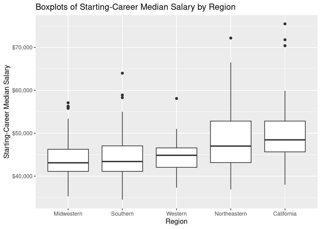
First we perform an ANOVA test for the Median Starting salary by comparing it to the regions. Below is a box-plot graph that shows the distribution of Staring Median Salary by Region. we can see that there is a visual difference in the distribution of starting median salaries that mostly differentiates the Northeastern and California region from the rest. These 2 regions have an apparent greater median starting Salary. There is still no statistical evidence that the mean median starting salary is associated with the regions, therefore we will perform ANOVA test to understand if there is a significant association between median staring salary and region.
Response: Starting.Median.Salary (numeric)
Explanatory: Region (factor)
Null Hypothesis: independence
# A tibble: 1 × 1
   stat
  <dbl>
1  11.7
Warning: Check to make sure the conditions have been met for the theoretical
method. {infer} currently does not check these for you.Warning: The dot-dot notation (`..density..`) was deprecated in ggplot2 3.4.0.
ℹ Please use `after_stat(density)` instead.
ℹ The deprecated feature was likely used in the infer package.
Please report the issue at <https://github.com/tidymodels/infer/issues>.Warning in min(diff(unique_loc)): no non-missing arguments to min; returning Inf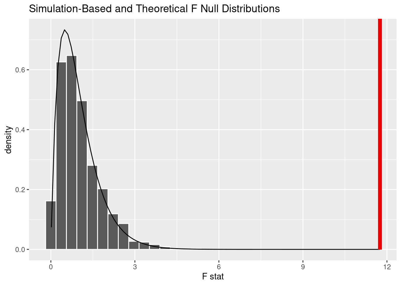
Warning: Please be cautious in reporting a p-value of 0. This result is an
approximation based on the number of `reps` chosen in the `generate()` step. See
`?get_p_value()` for more information.
# A tibble: 1 × 1
p_value
<dbl>
1 0After performing an ANOVA-test for differences in mean median starting salary, we found the observed F-statistic was 11.7494094. We then compared the F-statistic to a null distribution, generated under the assumption that median starting salary and Region are not actually related, to get a sense of how likely it would be for us to see this observed statistic if there were actually no association between the two variables.
We found that the p-value, or the probability we observed this F-statistic if there was no association between Median Starting-Salary and Region is less than 0.0001, Very Low. This is also evident in the simulated based-null distribution plot (shown above), since non of the simulated have an F-Statistic as large as the one calculated (11.74). Therefore we can reject the null hypothesis, that states that there is no association between Starting Salary and Region. There is enough statistical evidence to state that there is an association between Starting Salary and Region.
ANOVA Test for Median Mid-Career Salary and Region
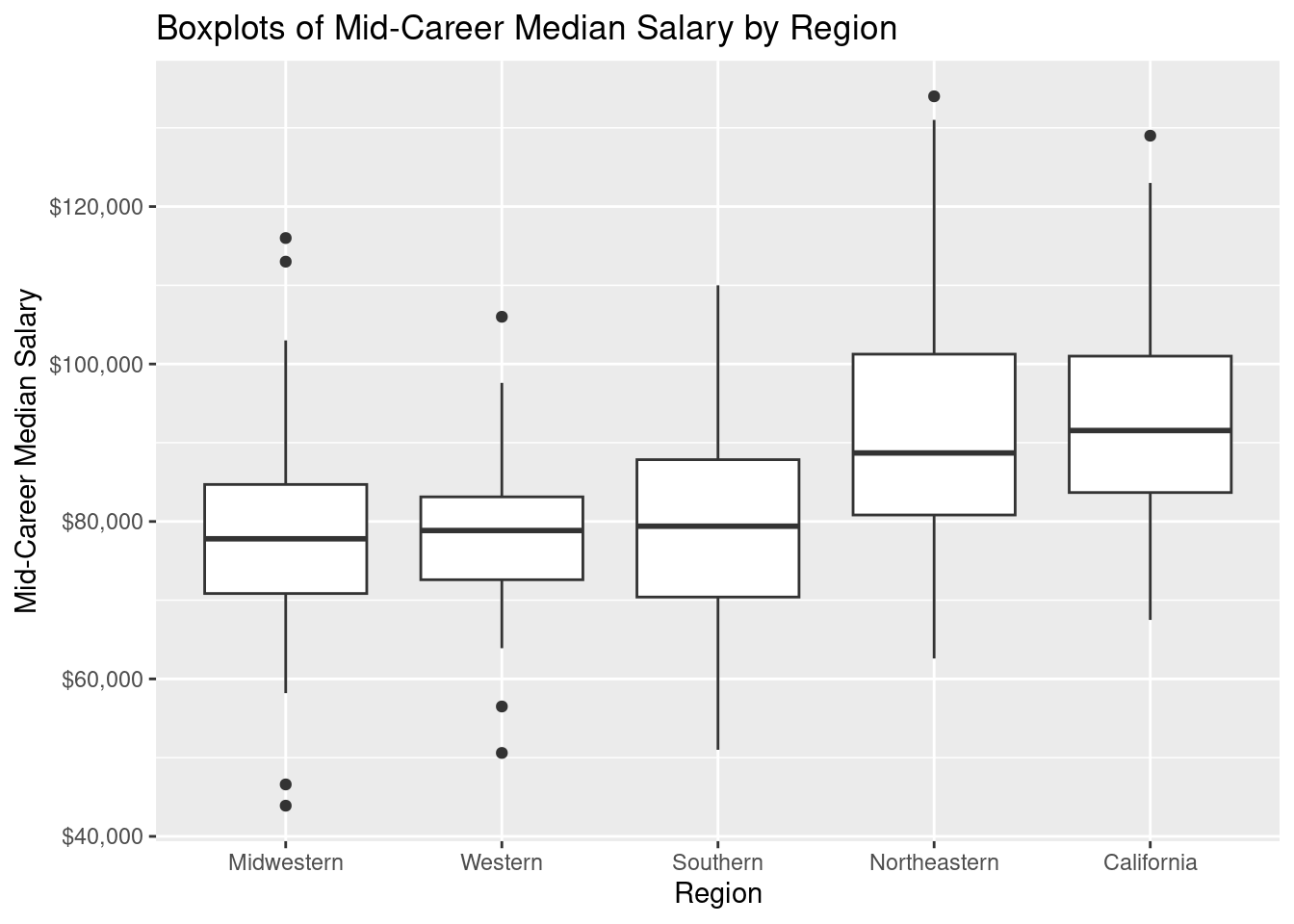
Next we assess whether there is a relationship between median mid-career salary and Region. The boxplots below help visualize the distribution of median salaries by region. If there was no relationship between mid-career salary and region we would expect box plots to line up along y-axis. It is apparent that some regions like the Northeast and California have a different distributions with higher mid-career salaries than other regions such as Mid-western and western region. There is still no statistical evidence that the mean median salary is different for all the regions, therefore we will perform ANOVA test to understand if there is a significant association between median mid-career salary and region.
Response: Mid.Career.Median.Salary (numeric)
Explanatory: Region (factor)
Null Hypothesis: independence
# A tibble: 1 × 1
stat
<dbl>
<<<<<<< HEAD
1 17.1Warning: Check to make sure the conditions have been met for the theoretical
method. {infer} currently does not check these for you.Warning: The dot-dot notation (`..density..`) was deprecated in ggplot2 3.4.0.
ℹ Please use `after_stat(density)` instead.
ℹ The deprecated feature was likely used in the infer package.
Please report the issue at <https://github.com/tidymodels/infer/issues>.Warning in min(diff(unique_loc)): no non-missing arguments to min; returning Inf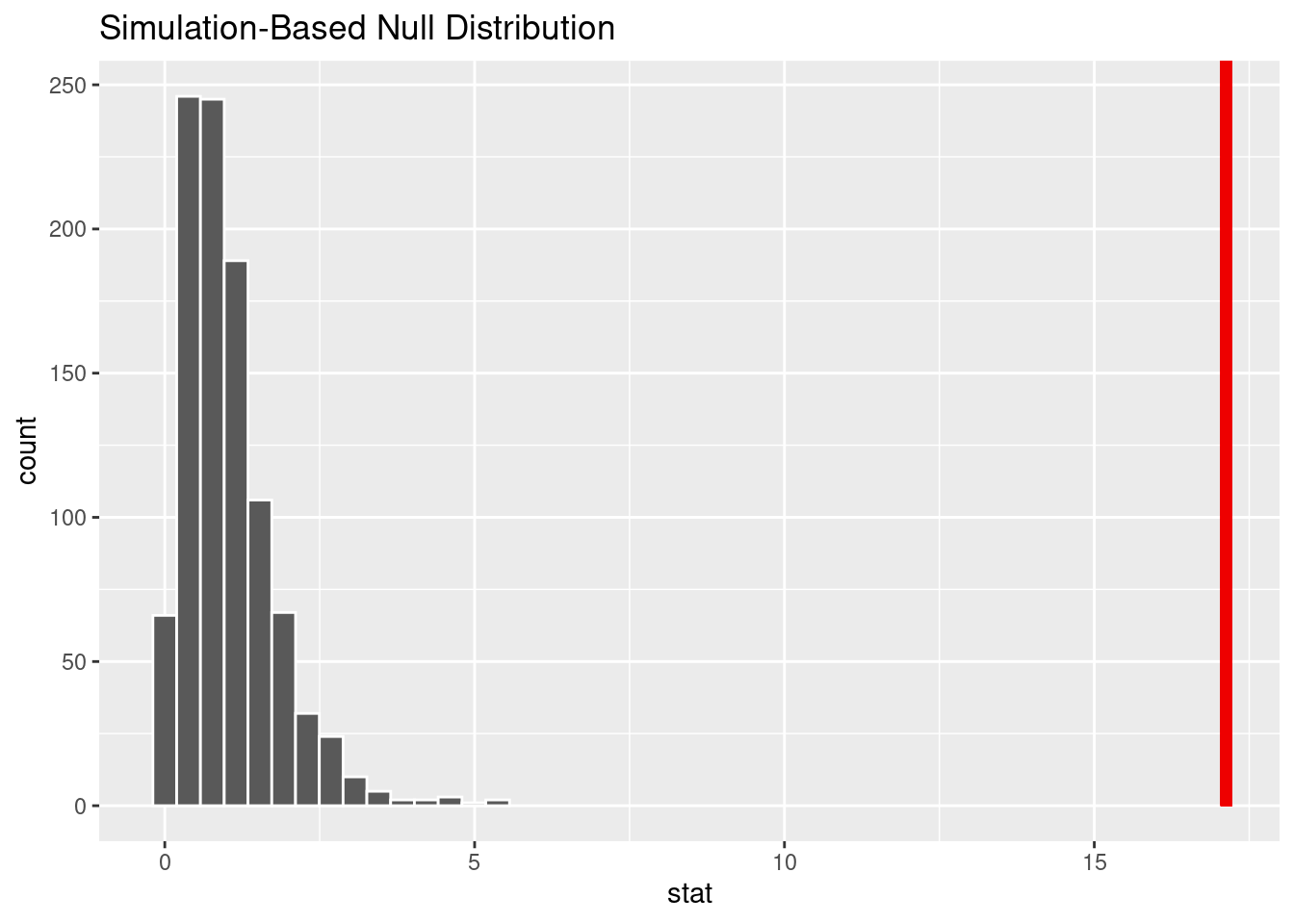
Warning: Please be cautious in reporting a p-value of 0. This result is an
approximation based on the number of `reps` chosen in the `generate()` step. See
`?get_p_value()` for more information.# A tibble: 1 × 1
p_value
<dbl>
1 0After performing an ANOVA-test for differences in mean median mid-career salary, we found the observed F-statistic was 17.129754 . We then compared the F-statistic to a null distribution, generated under the assumption that median mid-career salary and Region are not actually related, to get a sense of how likely it would be for us to see this observed statistic if there were actually no association between the two variables.
We found that the p-value, or the probability we observed this F-statistic if there was no association between median mid-career salary and Region is less than 0.0001, Very Low. This is also evident in the simulated based-null distribution plot (seen above), since non of the simulated have an F-Statistic as large as the one calculated. Therefore we can reject the null hypothesis, that states that there is no association between mid-career salary and Region. There is enough statistical evidence to state that there is an association between mid-career salary and Region.
School Type vs. Differences in Salaries
We are interested in whether there is a statistical significance at \(\alpha = 0.05\) in the difference between median salaries of different school types.
Median Starting Salary: Ivy League vs. State Schools
We will first analyze whether there is a statistical significance at \(\alpha = 0.05\) in the difference between Ivy League and State school median starting salaries.
\[ H_0: \mu_{ivy} - \mu_{state} = 0\\ H_A: \mu_{ivy} - \mu_{state} \neq 0 \]
Warning: Please be cautious in reporting a p-value of 0. This result is an
approximation based on the number of `reps` chosen in the `generate()` step. See
`?get_p_value()` for more information.# A tibble: 1 × 1
p_value
<dbl>
1 0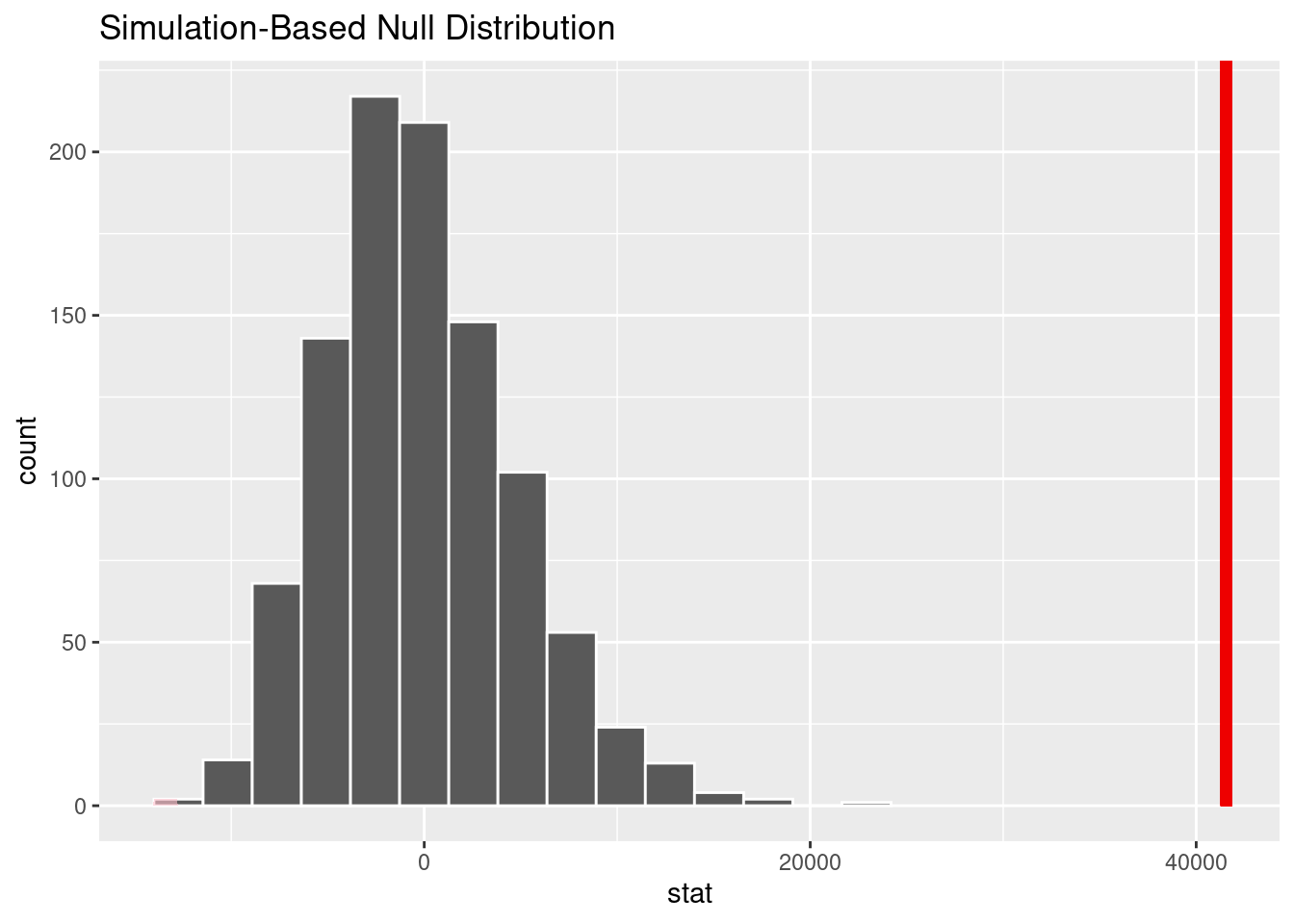
The p-value is 0, so we reject the null hypothesis. There is a significant difference in median starting salary between Ivy League and State schools.
Median Mid-Career Salary: Ivy League vs. State Schools
Next we analyze whether there is a statistical significance at \(\alpha = 0.05\) in the difference between Ivy League and State school median mid-career salaries. To accomplish this, we run a p-test between the median mid-career salaries for Ivy League colleges and state colleges.
\[ H_0: \mu_{ivy} - \mu_{state} = 0\\ H_A: \mu_{ivy} - \mu_{state} \neq 0 \]
Warning: Please be cautious in reporting a p-value of 0. This result is an
approximation based on the number of `reps` chosen in the `generate()` step. See
`?get_p_value()` for more information.# A tibble: 1 × 1
p_value
<dbl>
1 0
The p-value is 0, so we reject the null hypothesis. There is a significant difference in median mid-career salary between Ivy League and State schools.
Median Starting Salary: Ivy League vs. Engineering Schools
We are also interested in whether there is a statistical significance at \(\alpha = 0.05\) in the difference between median starting salaries of Ivy League and Engineering schools.
$$ H_0: *{ivy} -* = 0\
H_A: *{ivy} -* $$
# A tibble: 1 × 1
  p_value
    <dbl>
1 0.604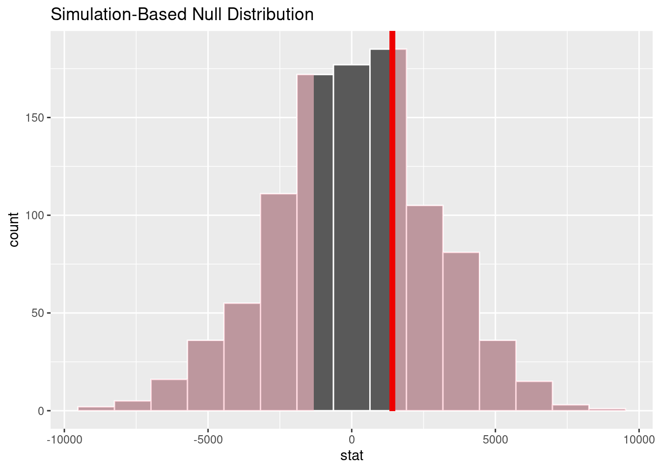
The p-value is 0.658, so we fail to reject the null hypothesis. There is insufficient evidence to conclude that there is a significance difference in median starting salary between Engineering and Ivy League schools.
Median Mid-Career Salary: Ivy League vs. Engineering Schools
Next we analyze whether there is a significant difference in median mid-career salary between Engineering and Ivy League schools.
$$ H_0: -* = 0\
H_A: -* $$
# A tibble: 1 × 1
  p_value
    <dbl>
1 0.006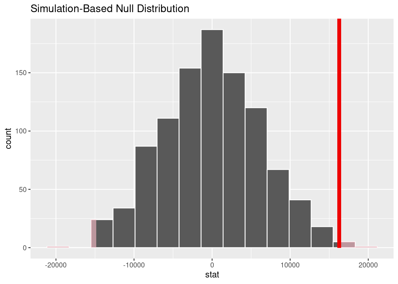
The p-value is 0.004, so we reject the null hypothesis. There is sufficient evidence to conclude that there is a significance difference in median mid-career salary between Engineering and Ivy League schools.
Interpretation and conclusions
When comparing the mean of median starting salaries at different types of schools, Engineering and Ivy League schools have a higher median starting salary than Liberal Arts, Party, and State schools. However, this measure equalizes over the course of one’s career, and the mean mid-career salaries of Engineering, Liberal Arts, Party, and State schools are more comparable. The mean mid-career salary measures of Ivy League schools are much higher than the other types of schools, with the mean 90th percentile measure of nearly $270,000 dwarfing the rest of the school types, whose mean 90th percentile salary are all under $200,000. This sets the Ivy League schools apart when it comes to mid-career earning potential. Note that this result can also be attributed to sample size: there are only eight Ivy League colleges, while other college types include many more colleges.
When comparing the mean of aggregate salary measures across different regions, the small differences in the mean median starting salary between regions becomes magnified as careers progress from starting salary to mid-career salary.
We analyze the difference between different regions with an ANOVA test. The p-values when analyzing the median starting and mid-career salaries for different college regions were both below 0.0001, so we are confident in rejecting the null hypotheses and concluding that there is an association between starting salary and college region, and mid-career salary and college region. Part of this conclusion can be attributed to the general trend of living costs and salary across different regions of the U.S. in general, as many college graduates seek jobs close to where they attended college.
When examining median salaries of graduates of different types of schools, there is significant (p < 0.0001) evidence to conclude that the median salary of graduates from Ivy League schools is different from graduates from State schools, for both starting and mid-career salaries. When comparing Ivy League and Engineering Schools, there is no significant different between median starting salaries, but at the mid-career levels, there is significant (p < 0.05) evidence that Ivy League median mid-career salaries is different than that of Engineering schools. This indicates that Ivy League schools have a greater earning potential at later career stages compared to Engineering schools. This could be due to many factors, including the different distribution of salaries across different college majors, and the representation of different college majors at each school.
Limitations
One major limitation is that data is self-reported, and may not be an accurate representation of all salaries, especially of graduates whose salaries were lower than their peers. Thus, there may be a self-reporting bias where graduates may inflate their salaries due to societal pressure of what they think they should be earned at a given point in their career. This could impact our conclusions as it can skew the analysis on salaries by type of college, if the data is not accurate.
Another limitation is the presence of a sampling bias. Obviously our datasets don’t include salary stats from every single graduate from every single university, and we were limited to the information that graduates chose to disclose. Again, graduates with lower salaries may be less likely to report while individuals with higher salaries may be more likely to report, particularly those who graduated from elite institutions where high salaries and success is expected, such as Ivy League or Engineering schools, leading to a skewed distribution of reported salaries. If our dataset is indeed biased towards higher salaries, our statistical analysis may then falsely show that attending an Ivy League school has a stronger effect on median salaries than it actually does.
Acknowledgments
None noted.