Project title

Report

Introduction

We looked at data collected by Alana Rhone from the Economic Research Service (ERS) in 2020, which gave us information on the food accessibility of different populations from counties all over the USA.
The research question we are trying to answer is: What is the impact of distance to supermarkets and grocery stores on the food accessibility and food security of low-income households in low population counties of New York? (Insert main findings + summary of results)
(insert main finding and summary of results)

Data description

The observations will be the different counties, with an identifying state attribute (New York) and normalized low access low income percent for populations that are at a distance of ½, 1, 10, and 20 miles.
This dataset was created to look at the correlation between low income populations and those populations’ distance from a supermarket in all counties in New York.
The dataset is funded by a food Access CSV File from the CORGIS Dataset Project by Ryan Whitcomb, Joung Min Choi, Bo Guan.
One process that might have influenced the data was what the surveyor’s definition of low-income, low-access is. Our conclusion on food accessibility and security is based on variables that indicate food insecurity rather than prove food insecurity. No collection of data of individual’s meals, school or government provided food was recorded. We can assume that factors such as having low income or being a far distance from a grocery store will cause food insecurity, but we do not know if there are other factors in these people’s lives preventing food insecurity, such as free and reduced school lunch programs, soup kitchens, and farmland prevalence.
The preprocessing that was done was a count of the population that was deemed low-income and an analysis of the distance of population from supermarkets.
The data was collected from a 2010 census so the participants were aware of the data collection, but there was no indication that the people who had data collected from them knew what they were used for.

Data analysis 1

library(tidyverse)

── Attaching packages ─────────────────────────────────────── tidyverse 1.3.2 ──
✔ ggplot2 3.4.1     ✔ purrr   1.0.0
✔ tibble  3.2.1     ✔ dplyr   1.1.2
✔ tidyr   1.2.1     ✔ stringr 1.5.0
✔ readr   2.1.3     ✔ forcats 0.5.2
── Conflicts ────────────────────────────────────────── tidyverse_conflicts() ──
✖ dplyr::filter() masks stats::filter()
✖ dplyr::lag()    masks stats::lag()

library(tidymodels)

── Attaching packages ────────────────────────────────────── tidymodels 1.0.0 ──
✔ broom        1.0.2     ✔ rsample      1.1.1
✔ dials        1.1.0     ✔ tune         1.1.1
✔ infer        1.0.4     ✔ workflows    1.1.2
✔ modeldata    1.0.1     ✔ workflowsets 1.0.0
✔ parsnip      1.0.3     ✔ yardstick    1.1.0
✔ recipes      1.0.6     
── Conflicts ───────────────────────────────────────── tidymodels_conflicts() ──
✖ scales::discard() masks purrr::discard()
✖ dplyr::filter()   masks stats::filter()
✖ recipes::fixed()  masks stringr::fixed()
✖ dplyr::lag()      masks stats::lag()
✖ yardstick::spec() masks readr::spec()
✖ recipes::step()   masks stats::step()
• Search for functions across packages at https://www.tidymodels.org/find/

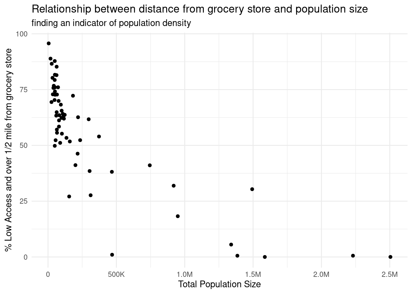
library(broom)
library(skimr)

food_access <- read_csv(file = "data/food_access.csv", show_col_types = FALSE)

a1_data <- food_access |>
  filter(State == "New York") |>
  # select relevant variables
  select(County, 
         State, 
         Population, 
         `Low Access Numbers.People.1 Mile`, 
         `Low Access Numbers.People.10 Miles`, 
         `Low Access Numbers.People.20 Miles`) |>
  # calculate % of pop that is low access and lives >0.5m from grocery store
    mutate(
    `20` = `Low Access Numbers.People.20 Miles`,
    `10` = `Low Access Numbers.People.10 Miles` - `Low Access Numbers.People.20 Miles`,
    `1` = `Low Access Numbers.People.1 Mile` - `Low Access Numbers.People.10 Miles`
  ) |>
  mutate(`% Low Access >.5m` = 
    100*(`1` + 
         `10` +
         `20`)/Population) |>
  # take out raw population numbers
    select(County, 
         State, 
         Population, 
         `% Low Access >.5m`)

# scatter plot
    a1_data |>
      ggplot(aes(x = Population, y = `% Low Access >.5m`)) +
      geom_point() +
      scale_x_continuous(labels = label_number_si()) +
      labs(x = "Total Population Size", 
           y = "% Low Access and over 1/2 mile from grocery store", 
           title = "Relationship between distance from grocery store and population size",
           subtitle = "finding an indicator of population density") +
           theme_minimal()

Warning: `label_number_si()` was deprecated in scales 1.2.0.
ℹ Please use the `scale_cut` argument of `label_number()` instead.

# add an exponential regression line
    # create a linear regression
a1_linear_fit <- linear_reg() |>
fit(`% Low Access >.5m` ~ Population, data = a1_data)
tidy(a1_linear_fit)

# A tibble: 2 × 5
  term          estimate  std.error statistic  p.value
  <chr>            <dbl>      <dbl>     <dbl>    <dbl>
1 (Intercept) 67.7       2.16            31.3 6.92e-39
2 Population  -0.0000367 0.00000352     -10.4 4.20e-15

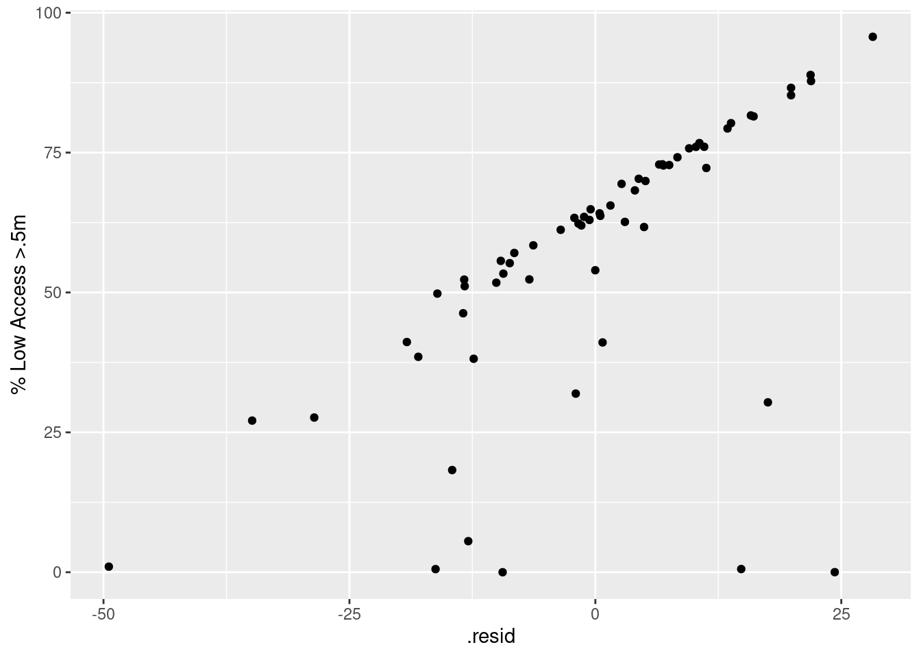
   # check that relationship is nonlinear with a residual plot
a1_resid <- a1_linear_fit |>
augment(a1_data)
a1_resid

# A tibble: 62 × 6
   County             State    Population `% Low Access >.5m` .pred .resid
   <chr>              <chr>         <dbl>               <dbl> <dbl>  <dbl>
 1 Albany County      New York     304204              38.5    56.5 -18.0 
 2 Allegany County    New York      48946              79.3    65.9  13.4 
 3 Bronx County       New York    1385108               0.556  16.8 -16.2 
 4 Broome County      New York     200600              41.1    60.3 -19.2 
 5 Cattaraugus County New York      80317              61.2    64.7  -3.52
 6 Cayuga County      New York      80026              58.4    64.7  -6.31
 7 Chautauqua County  New York     134905              53.4    62.7  -9.35
 8 Chemung County     New York      88830              51.1    64.4 -13.3 
 9 Chenango County    New York      50477              74.2    65.8   8.35
10 Clinton County     New York      82128              63.5    64.7  -1.15
# ℹ 52 more rows

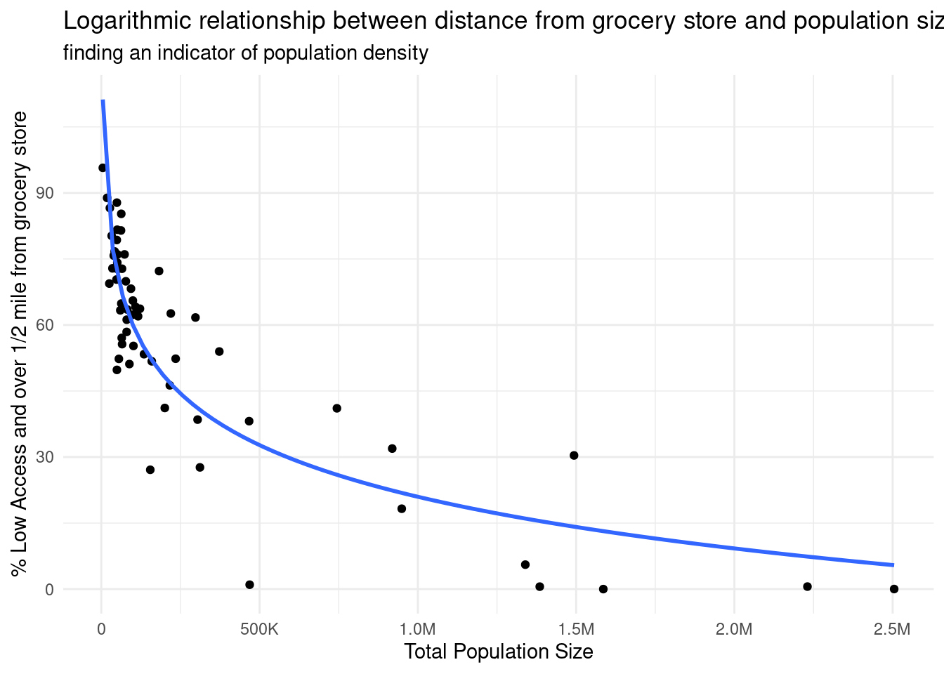
ggplot(a1_resid, aes(x = .resid, y = `% Low Access >.5m`)) +
  geom_point() # non-random results

   # scatter plot with exponential regression line
a1_data |>
  ggplot(aes(x = Population, y = `% Low Access >.5m`)) +
  geom_point() +
  scale_x_continuous(labels = label_number_si()) +
  geom_smooth(method = "lm", formula = y ~ log(x), se = FALSE) +
  labs(x = "Total Population Size",
       y = "% Low Access and over 1/2 mile from grocery store",
       title = "Logarithmic relationship between distance from grocery store and population size",
       subtitle = "finding an indicator of population density") +
  theme_minimal()

  # can repeat analysis with another variable to verify 
    # Notes:
    # - ~ 60 samples makes this a valid sample size
    # - Limitation: would be better if we could calculate % of total people living 1/2m from the grocery store instead of low access %

Evaluation of significance 1

Null hypothesis: There is no significant relationship between the % of a county’s population that is low access and living > 0.5 miles from a grocery store and the total population of a county.

\[H_0: r^2 < 0.7\]

Alternative hypothesis: There is a significant relationship between the % of a county’s population that is low access and living > 0.5 miles from a grocery store and the total population of a county.

\[H_A: r^2 > 0.7\]

# calculate R-squared value
a1_log_fit <- lm(`% Low Access >.5m` ~ log(Population), data = a1_data)
tidy(a1_log_fit)

# A tibble: 2 × 5
  term            estimate std.error statistic  p.value
  <chr>              <dbl>     <dbl>     <dbl>    <dbl>
1 (Intercept)        255.      13.4       19.0 4.12e-27
2 log(Population)    -16.9      1.13     -14.9 7.28e-22

ssr <- sum((predict(a1_log_fit) - mean(a1_data$`% Low Access >.5m`))^2)
sst <- sum((a1_data$`% Low Access >.5m` - mean(a1_data$`% Low Access >.5m`))^2)
rsq <- ssr/sst
rsq

[1] 0.787824

# display conslusion
if(rsq >= 0.7){
  cat("Based on the r squared value, we reject the null hypothesis. There is a significant relationship between the % of a county's population that is low access and living > 0.5 miles from a grocery store and the total population of a county. Therefore, we will assume that population size can be used as an indicator of population density for the purposes of this study.\n")
} else {
  cat("Based on the r squared value, we fail to reject the null hypothesis. There is no significant relationship between the % of a county's population that is low access and living > 0.5 miles from a grocery store and the total population of a county. Therefore, we will not assume that population size can be used as an indicator of population density for the purposes of this study.\n")
}

Based on the r squared value, we reject the null hypothesis. There is a significant relationship between the % of a county's population that is low access and living > 0.5 miles from a grocery store and the total population of a county. Therefore, we will assume that population size can be used as an indicator of population density for the purposes of this study.

Data analysis 2

fa_ny <- food_access |>
  filter(State == "New York") |> 
  mutate(
    County = str_replace(string = County, pattern = "County", replacement = ""),
    `20` = `Low Access Numbers.People.20 Miles`,
    `10` = `Low Access Numbers.People.10 Miles` - `Low Access Numbers.People.20 Miles`,
    `1` = `Low Access Numbers.People.1 Mile` - `Low Access Numbers.People.10 Miles`,
    `0.5` = `Low Access Numbers.People.1/2 Mile` - `Low Access Numbers.People.1 Mile`
  ) |>
  select(County, Population, `0.5`, `1`, `10`, `20`) |> 
  pivot_longer(
    cols = c(`0.5`, `1`, `10`, `20`), 
    names_to = "Distance") |>
  mutate(Distance = as.factor(Distance)) |>
  arrange(desc(Population))
fa_ny

# A tibble: 248 × 4
   County      Population Distance  value
   <chr>            <dbl> <fct>     <dbl>
 1 "Kings "       2504700 0.5       40467
 2 "Kings "       2504700 1           394
 3 "Kings "       2504700 10            0
 4 "Kings "       2504700 20            0
 5 "Queens "      2230722 0.5      134309
 6 "Queens "      2230722 1         12724
 7 "Queens "      2230722 10            0
 8 "Queens "      2230722 20            0
 9 "New York "    1585873 0.5         473
10 "New York "    1585873 1             2
# ℹ 238 more rows

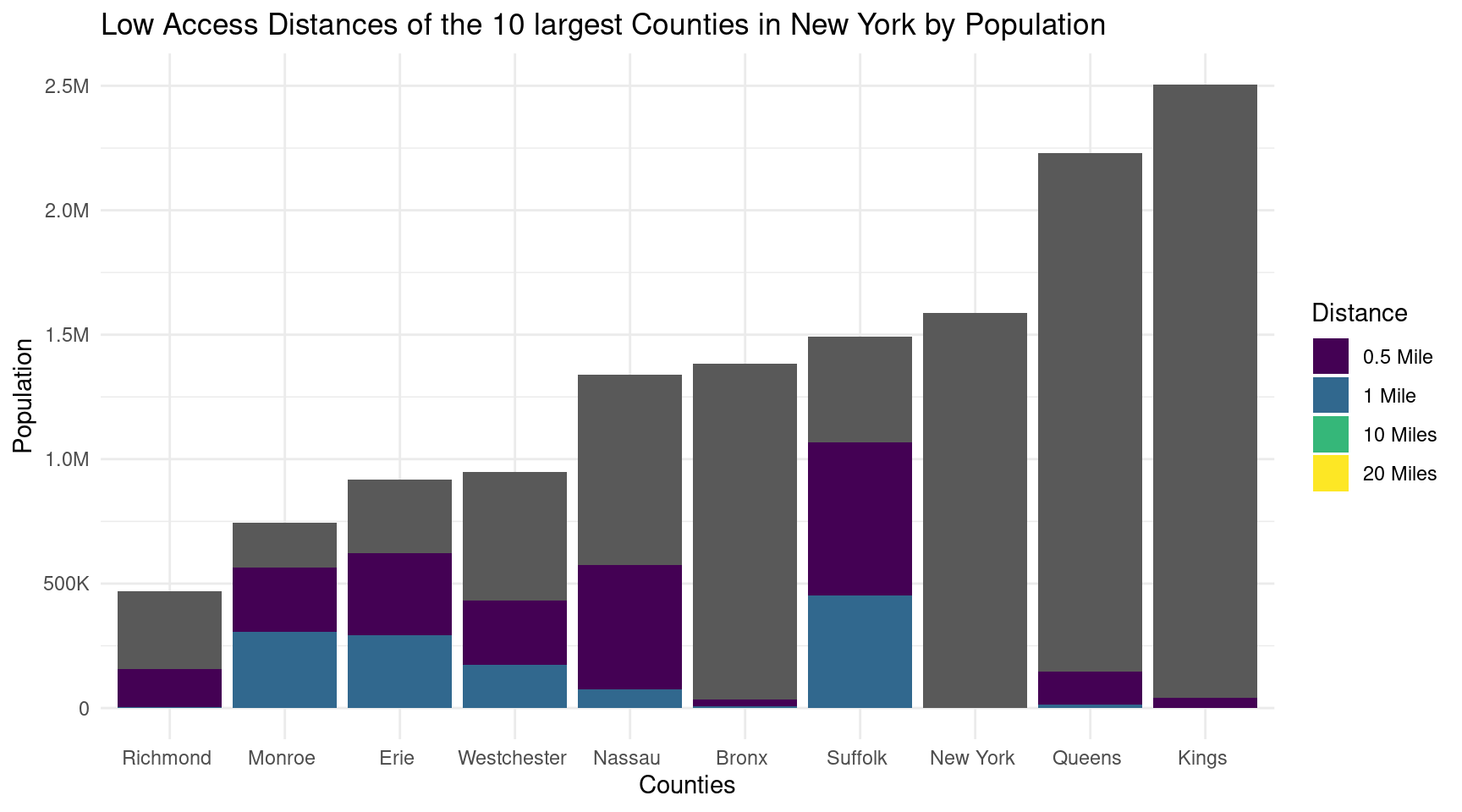
 head(fa_ny, 40) |>
   ggplot(aes(x = reorder(County, Population), y = Population/4)) + 
   geom_bar(stat = "identity") +
   geom_bar(
     aes(x = County, y = value, fill = Distance), 
     position = "stack", 
     stat = "identity") + 
   scale_y_continuous(labels = label_number_si()) +
   scale_fill_viridis_d(labels = c("0.5 Mile", "1 Mile", "10 Miles", "20 Miles")) +
   labs(
     x = "Counties",
     y = "Population",
     title = "Low Access Distances of the 10 largest Counties in New York by Population"
   ) + 
   theme_minimal()

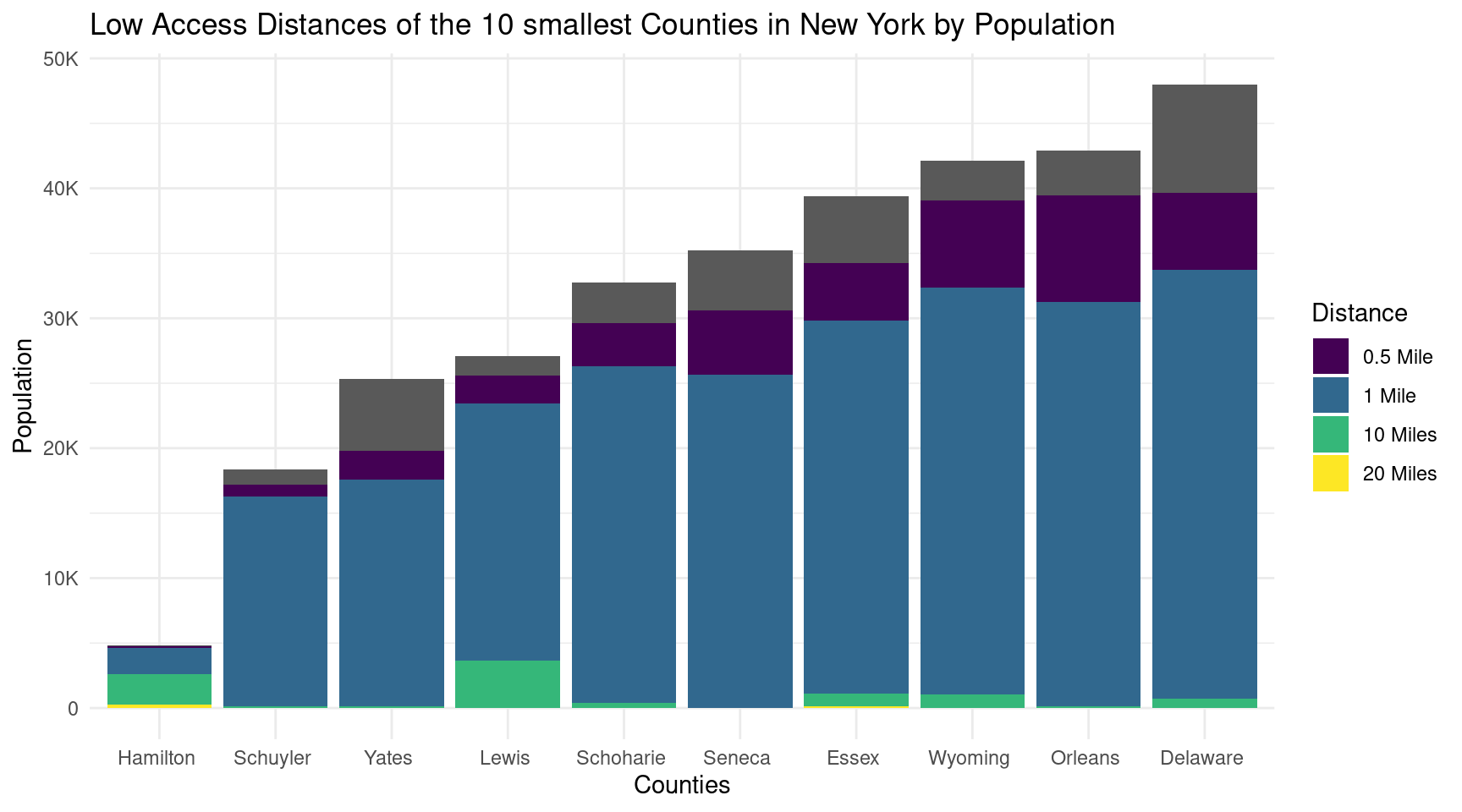
 tail(fa_ny, 40) |>
 ggplot(aes(x = reorder(County, Population), y = Population/4)) + 
   geom_bar(stat = "identity") +
   geom_bar(
     aes(x = County, y = value, fill = Distance), 
     position = "stack", 
     stat = "identity") + 
   # geom_text(aes(x = County, y = Population, label = Population)) + 
   scale_y_continuous(labels = label_number_si()) +
   scale_fill_viridis_d(labels = c("0.5 Mile", "1 Mile", "10 Miles", "20 Miles")) +
   labs(
     x = "Counties",
     y = "Population",
     title = "Low Access Distances of the 10 smallest Counties in New York by Population"
   ) + 
   theme_minimal()

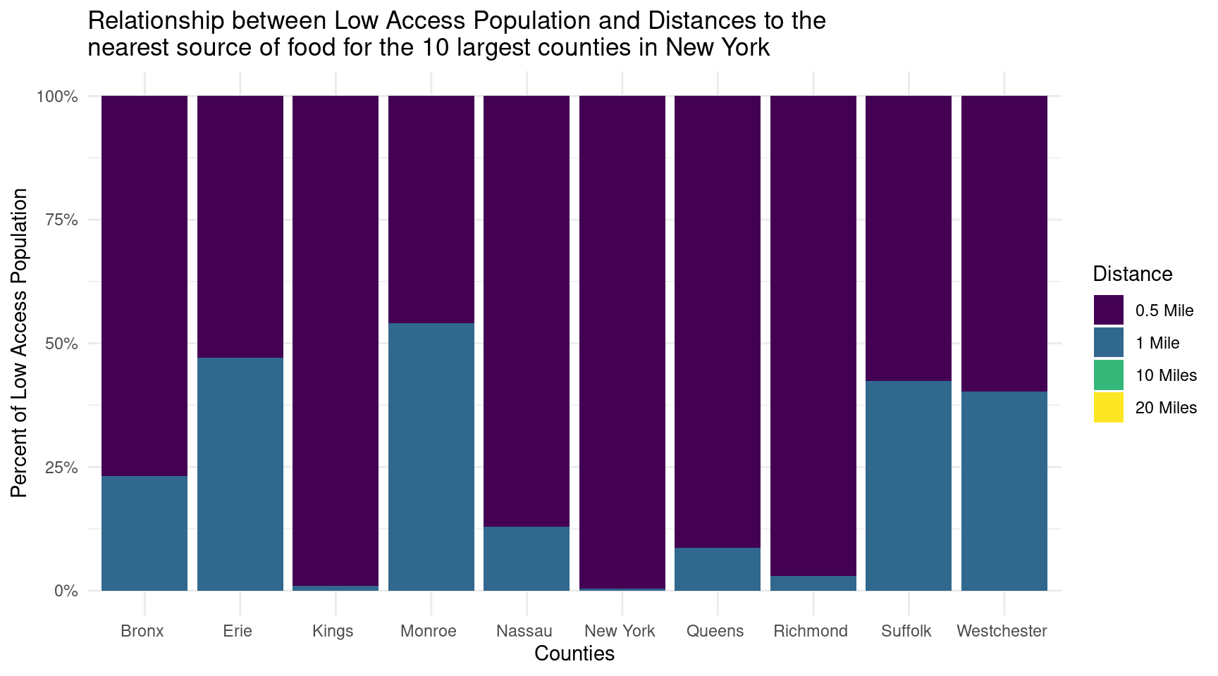
head(fa_ny, 40) |>
  ggplot(aes(x = reorder(County, Population), y = Population/4)) + 
  geom_bar(
    aes(x = County, y = value, fill = Distance), 
    position = "fill", 
    stat = "identity") + 
  scale_y_continuous(labels = scales::percent) +
  scale_fill_viridis_d(labels = c("0.5 Mile", "1 Mile", "10 Miles", "20 Miles")) +
  labs(
    x = "Counties",
    y = "Percent of Low Access Population",
    title = "Relationship between Low Access Population and Distances to the \nnearest source of food for the 10 largest counties in New York"
  ) + 
  theme_minimal()

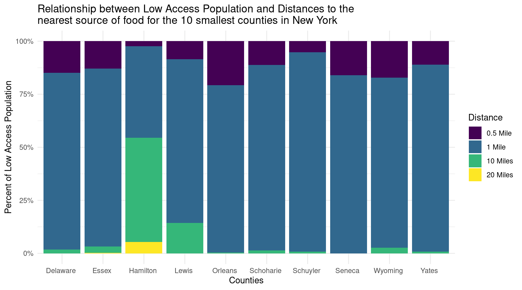
tail(fa_ny, 40) |>
ggplot(aes(x = reorder(County, Population), y = Population/4)) + 
  geom_bar(
    aes(x = County, y = value, fill = Distance), 
    position = "fill", 
    stat = "identity") + 
  scale_y_continuous(labels = scales::percent) +
  scale_fill_viridis_d(labels = c("0.5 Mile", "1 Mile", "10 Miles", "20 Miles")) +
  labs(
    x = "Counties",
    y = "Percent of Low Access Population",
    title = "Relationship between Low Access Population and Distances to the \nnearest source of food for the 10 smallest counties in New York"
  ) + 
  theme_minimal()

Evaluation of significance 2

Null hypothesis: There is no significant relationship between the % of a county’s population that is low access and living > 0.5 miles from a grocery store and the size of a county.

Alternative hypothesis: There is a significant relationship between the % of a county’s population that is low access and living > 0.5 miles from a grocery store and the size of a county.

Interpretation and conclusions

We found that we can reliably use population size as an indicator of whether a county is rural or urban by comparing population size of counties with the percentage of county total population that lives over half a mile from a grocery store. As we were doing the data analysis, we used a scatter plot to visualize the relationship, with the percentage of total population that lives over half a mile from the grocery store on the y axis, and the total population size on the x axis. Based on the R-squared value of 0.7985, we can say that there is a high level of correlation given that 0.7985 is greater than 0.7. However, since the R-squared value is not 0.9 or above, it is not the most reliable model that exists. Moreover, we were intrigued how the relatinoship is not linear, but rather logarithmic. This suggests diminishing returns or decreasing growth, instead a linear relationship that suggests a constant proportional relationship between total population size and low access individuals over 0.5 miles to the grocery store.

The stacked bar charts comparing the largest and smallest 10 counties in New York indicate that the smallest counties have a higher proportion of residents living farther away from grocery stores, resulting in a larger low access population. This suggests potential disparities in food accessibility, highlighting the need for targeted interventions and policies to improve access to fresh food in these areas.

Limitations

The dataset has geographic bias, as it only covers the United States at the county level and does not provide information on specific types of food sources. As such, this data may not be generalizable to other regions.
The data may not reflect actual availability or nutritional value and was last updated in 2015.
Furthermore, it relies on self-reported data from retailers and lacks qualitative information like information on cultural and social barriers to accessing healthy food, perceptions of food quality and availability, and the impact of food insecurity on health outcomes and well-being. This information gap limits the dataset’s usefulness in understanding the experiences and perspectives of individuals and communities.
The dataset focuses on accessibility to supermarkets, supercenters, and grocery stores, which are more commonly found in urban areas, potentially overlooking the food access issues faced by rural communities.
The dataset includes measures of individual-level resources, such as family income, which could bias the conclusions towards income-based food access disparities and overlook other contributing factors.
The dataset assumes that the food available at supermarkets and grocery stores is healthy, which may not always be the case.
Finally, the dataset does not account for the nutritional quality or availability of specific food items, which could impact the conclusions drawn regarding food access and health outcomes.

Acknowledgments

Lecture slides made by Professor Soltoff provided concepts used in this report, such as hypothesis tests, regressions, and more.