Marvelous Starmie
Report
Introduction
Our team is investigating the relationship between crime data and state allocation of spending. Our research question is analyzing whether state allocation of funds has a correlation with violent crime rates. The hypothesis is that states with more state funding for prisons, education, and the police tend to have lower violent crime rates.
Data description
Our dataset (finance_crime) combined columns of violent crime counts for each state between 2015-2019 with proportions of state spending for fields including prisons, education, and the police. Each row is the data for one state for a given year. Each state has 5 years, so there are 5 rows per state. We merged our data from the National Incident-Based Reporting System’s crime reports and state spending reports, so there are two different data sources.
The crime data was published by the Uniform Crime Reporting Program from the FBI, and was published to help provide comprehensive information surrounding police forces for research, analysis, and public use. The dataset was funded by the FBI and other parts of the government, with the data coming from official crime arrest records through a partnership with police forces/offices. Since the data is from official crime arrest records, the only reasonable factor influencing data collection would be underlying biases leading to the arrests. The people involved most likely did not expect their data to be used for public research, but most likely were aware of the data collection. The Crime Reporting Program most likely put the comprehensive data together themselves after gaining the numbers from each county. When our group tried to use the data, each year was separated, so we had to merge each year and select the necessary columns and rows from each dataframe. We also had to drop NA values, and calculate the violence rate, because only totals were given.
The state spending reports come from the United States Census Bureau, with the reports therefore being funded by the government. The data was collected and created by the Census Bureau, and the state governments representatives acting as respondents were aware of the data collection and what t would be used for. This data was created to aid with policy research, GDP estimates, for other government agencies, and for educational purposes. Our group received the spending data and had to undergo a similar process as the previous dataset to clean it before being able to merge both the crime and spending data.
Data analysis
Rows: 250 Columns: 13
── Column specification ────────────────────────────────────────────────────────
Delimiter: ","
chr  (1): State
dbl (12): Year, Population, Total_Revenue, Correction, Education, Health, We...

ℹ Use `spec()` to retrieve the full column specification for this data.
ℹ Specify the column types or set `show_col_types = FALSE` to quiet this message.
[1] 0.1565091[1] 0.002084022[1] 0.3096611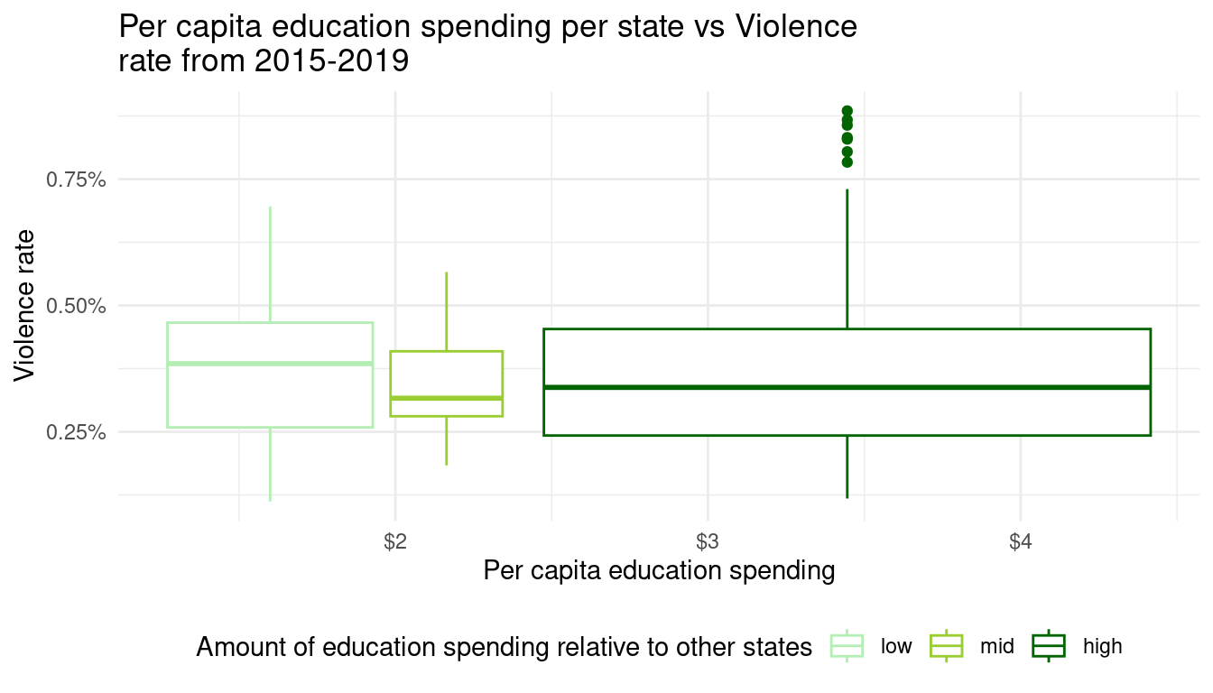
The correlation value between per capita education spending and violence rate is 0.002084022, which indicates a very weak correlation. This weak correlation is evident in the boxplot visualization above, where states with a ‘mid’ quantity of education spending have a significantly lower median violence rate (0.27%) than states with a ‘high’ quantity of education spending (0.30%). This data is contrary to our hypothesis, because if it were consistent, we would expect the violence rate to decrease instead of increase as education spending increases.
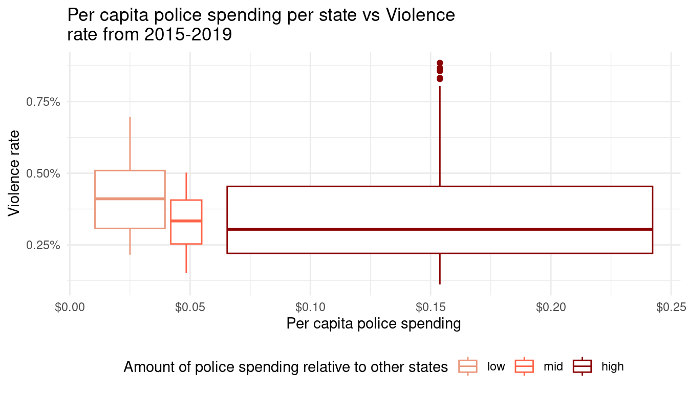
The correlation value between per capita police spending and violence rate is 0.1565091, which indicates a weak positive correlation, although significantly stronger than police spending’s correlation. Based on the boxplot visualization above, states with a ‘low’ quantity of police spending (0.4%) have a higher median violence rate than median violence rate of the states with a ‘mid’ quantity of police spending (0.3%), which have a significantly lower median violence rate than states with a ‘high’ quantity of police spending (0.27%). This data is consistent with our hypothesis, because the violence rate sequentially decreases as police spending increases. However, it’s important to note that the correlation is still considered weakly positive, and there may be other factors that contribute to this trend.
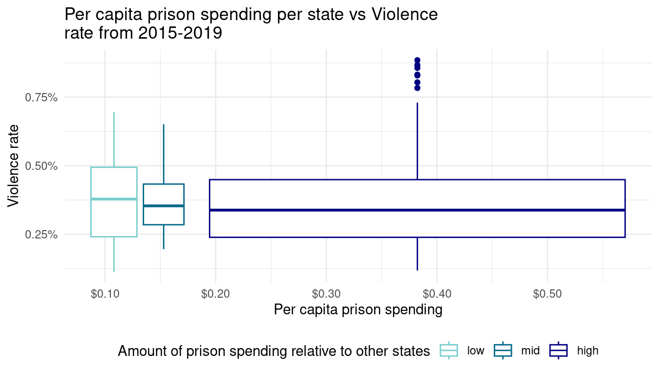
The correlation value between per capita prison spending and violence rate is 0.3096611, which indicates a small positive correlation, which is significantly stronger than both police and education spending’s correlation. Based on the boxplot visualization above, states with a ‘low’ quantity of prison spending (0.375%) have a higher median violence rate than median violence rate of the states with a ‘mid’ quantity of prison spending (0.35%), which have a significantly lower median violence rate than states with a ‘high’ quantity of prison spending (0.27%). This boxplot is representative of our hypothesis, because the violence rate decreases as prison spending increases. However, even though this correlation is considered the highest of the three sectors, the positive correlation is not significant enough to say that there is a significant correlation, so there are likely other factors contributing to the boxplot’s presentation of decreasing median violence rates.
##Linear Model
Call:
lm(formula = Violent_Rate ~ percap_prison, data = finance_crime)

Residuals:
       Min         1Q     Median         3Q        Max
-0.0029664 -0.0009922 -0.0001928  0.0007387  0.0044274

Coefficients:
               Estimate Std. Error t value Pr(>|t|)
(Intercept)   0.0025574  0.0002393  10.688  < 2e-16 ***
percap_prison 0.0068563  0.0013369   5.129 5.89e-07 ***
---
Signif. codes:  0 '***' 0.001 '**' 0.01 '*' 0.05 '.' 0.1 ' ' 1

Residual standard error: 0.001406 on 248 degrees of freedom
Multiple R-squared:  0.09589,   Adjusted R-squared:  0.09224
F-statistic:  26.3 on 1 and 248 DF,  p-value: 5.885e-07
Call:
lm(formula = Violent_Rate ~ percap_edu, data = finance_crime)

Residuals:
       Min         1Q     Median         3Q        Max
-0.0025719 -0.0011950 -0.0001194  0.0007996  0.0051466

Coefficients:
             Estimate Std. Error t value Pr(>|t|)
(Intercept) 3.685e-03  3.682e-04  10.007   <2e-16 ***
percap_edu  5.158e-06  1.572e-04   0.033    0.974
---
Signif. codes:  0 '***' 0.001 '**' 0.01 '*' 0.05 '.' 0.1 ' ' 1

Residual standard error: 0.001478 on 248 degrees of freedom
Multiple R-squared:  4.343e-06, Adjusted R-squared:  -0.004028
F-statistic: 0.001077 on 1 and 248 DF,  p-value: 0.9738
Call:
lm(formula = Violent_Rate ~ percap_police, data = finance_crime)

Residuals:
       Min         1Q     Median         3Q        Max
-0.0031688 -0.0010605 -0.0000954  0.0008181  0.0047902

Coefficients:
               Estimate Std. Error t value Pr(>|t|)
(Intercept)   0.0033107  0.0001801  18.378   <2e-16 ***
percap_police 0.0065531  0.0026260   2.495   0.0132 *
---
Signif. codes:  0 '***' 0.001 '**' 0.01 '*' 0.05 '.' 0.1 ' ' 1

Residual standard error: 0.00146 on 248 degrees of freedom
Multiple R-squared:  0.0245,    Adjusted R-squared:  0.02056
F-statistic: 6.227 on 1 and 248 DF,  p-value: 0.01323
Call:
lm(formula = Violent_Rate ~ percap_prison + percap_edu + percap_police,
    data = finance_crime)

Residuals:
       Min         1Q     Median         3Q        Max
-0.0022304 -0.0011045 -0.0001721  0.0006560  0.0044675

Coefficients:
                Estimate Std. Error t value Pr(>|t|)
(Intercept)    0.0031154  0.0003759   8.288 7.52e-15 ***
percap_prison  0.0116561  0.0021776   5.353 1.99e-07 ***
percap_edu    -0.0004193  0.0001809  -2.318   0.0213 *
percap_police -0.0068776  0.0043622  -1.577   0.1162
---
Signif. codes:  0 '***' 0.001 '**' 0.01 '*' 0.05 '.' 0.1 ' ' 1

Residual standard error: 0.001379 on 246 degrees of freedom
Multiple R-squared:  0.137, Adjusted R-squared:  0.1264
F-statistic: 13.01 on 3 and 246 DF,  p-value: 6.451e-08
Call:
lm(formula = Violent_Rate ~ percap_prison * percap_edu * percap_police,
    data = finance_crime)

Residuals:
       Min         1Q     Median         3Q        Max
-0.0023054 -0.0008891 -0.0000250  0.0006738  0.0047092

Coefficients:
                                         Estimate Std. Error t value Pr(>|t|)
(Intercept)                             0.0148470  0.0021943   6.766 9.88e-11
percap_prison                          -0.0614422  0.0141342  -4.347 2.03e-05
percap_edu                             -0.0034030  0.0007952  -4.279 2.70e-05
percap_police                          -0.1797356  0.0376931  -4.768 3.21e-06
percap_prison:percap_edu                0.0198603  0.0051250   3.875 0.000137
percap_prison:percap_police             0.9520338  0.1897377   5.018 1.01e-06
percap_edu:percap_police                0.0432150  0.0116936   3.696 0.000271
percap_prison:percap_edu:percap_police -0.2518722  0.0558739  -4.508 1.02e-05

(Intercept)                            ***
percap_prison                          ***
percap_edu                             ***
percap_police                          ***
percap_prison:percap_edu               ***
percap_prison:percap_police            ***
percap_edu:percap_police               ***
percap_prison:percap_edu:percap_police ***
---
Signif. codes:  0 '***' 0.001 '**' 0.01 '*' 0.05 '.' 0.1 ' ' 1

Residual standard error: 0.001217 on 242 degrees of freedom
Multiple R-squared:  0.3385,    Adjusted R-squared:  0.3193
F-statistic: 17.69 on 7 and 242 DF,  p-value: < 2.2e-16
In this analysis, we compared five different models to understand the relationship between government spending on prisons, education, and police and the violent crime rate.
Prison Model: The prison_model shows that about 9.22% of the variation in the violent crime rate can be explained by per capita spending on prisons. The percap_prison variable is statistically significant (p < 0.001).
Education Model: The edu_model suggests that the percap_edu variable does not explain any variation in the violent crime rate, and it is not statistically significant (p = 0.974).
Police Model: In the police_model, approximately 2.056% of the variation in the violent crime rate can be explained by per capita spending on police. The percap_police variable is statistically significant (p = 0.0132).
Additive Model (pep_add_model): This model accounts for 12.64% of the variation in the violent crime rate by combining per capita prison, education, and police expenditure. It shows a significant positive relationship between violent crime rate and per capita prison expenditure (p < 0.001), a significant negative relationship between violent crime rate and per capita education expenditure (p = 0.0213), and no statistically significant relationship between violent crime rate and per capita police expenditure (p = 0.1162).
Interaction Model (pep_int_model): The interaction model explains approximately 31.93% of the variation in the violent crime rate by considering the interactions between the three variables. The model shows significant interaction effects between per capita prison, education, and police expenditure on the violent crime rate (p < 0.001), suggesting that their combined effect is significant and not independent of each other.
In conclusion, the interaction model (pep_int_model) has the highest adjusted R-squared value and reveals the complex relationships between government spending on prisons, education, and police in relation to the violent crime rate. This model suggests that it is crucial to consider the combined effects and interactions of these variables when analyzing their impact on violent crime.
Evaluation of significance
Hypothesis Test - Police
\[ H_0: p_c-p_p=0 \]
\[ H_A: p_c-p_p\neq0 \]
Null Hypothesis: There is no significant difference in violence rate in states with low per cap police spending and high per cap police spending.
Alternative Hypothesis: There is a significant difference in violence rate in states with low per cap police spending and high per cap police spending.
Warning: The statistic is based on a difference or ratio; by default, for
difference-based statistics, the explanatory variable is subtracted in the
order "high" - "low", or divided in the order "high" / "low" for ratio-based
statistics. To specify this order yourself, supply `order = c("high", "low")` to
the calculate() function.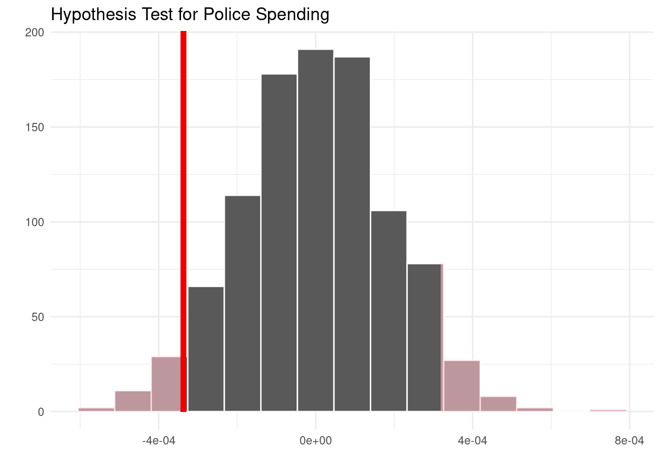
# A tibble: 1 × 1
  p_value
    <dbl>
1   0.078
Since the p-value is 0.078 which is greater than 0.05(95% significance level), we fail to reject the null hypothesis. The data does not provide convincing evidence that the average violence crime rates of states with low per cap police spending and high per cap police spending is different.
Hypothesis Test - Education
\[ H_0: p_c-p_e=0 \]
\[ H_A: p_c-p_e\neq0 \]
Null Hypothesis: There is no significant difference in violence rate in states with low per cap education spending and high per cap education spending.
Alternative Hypothesis: There is a significant difference in violence rate in states with low per cap education spending and high per cap education spending.
Warning: The statistic is based on a difference or ratio; by default, for
difference-based statistics, the explanatory variable is subtracted in the
order "high" - "low", or divided in the order "high" / "low" for ratio-based
statistics. To specify this order yourself, supply `order = c("high", "low")` to
the calculate() function.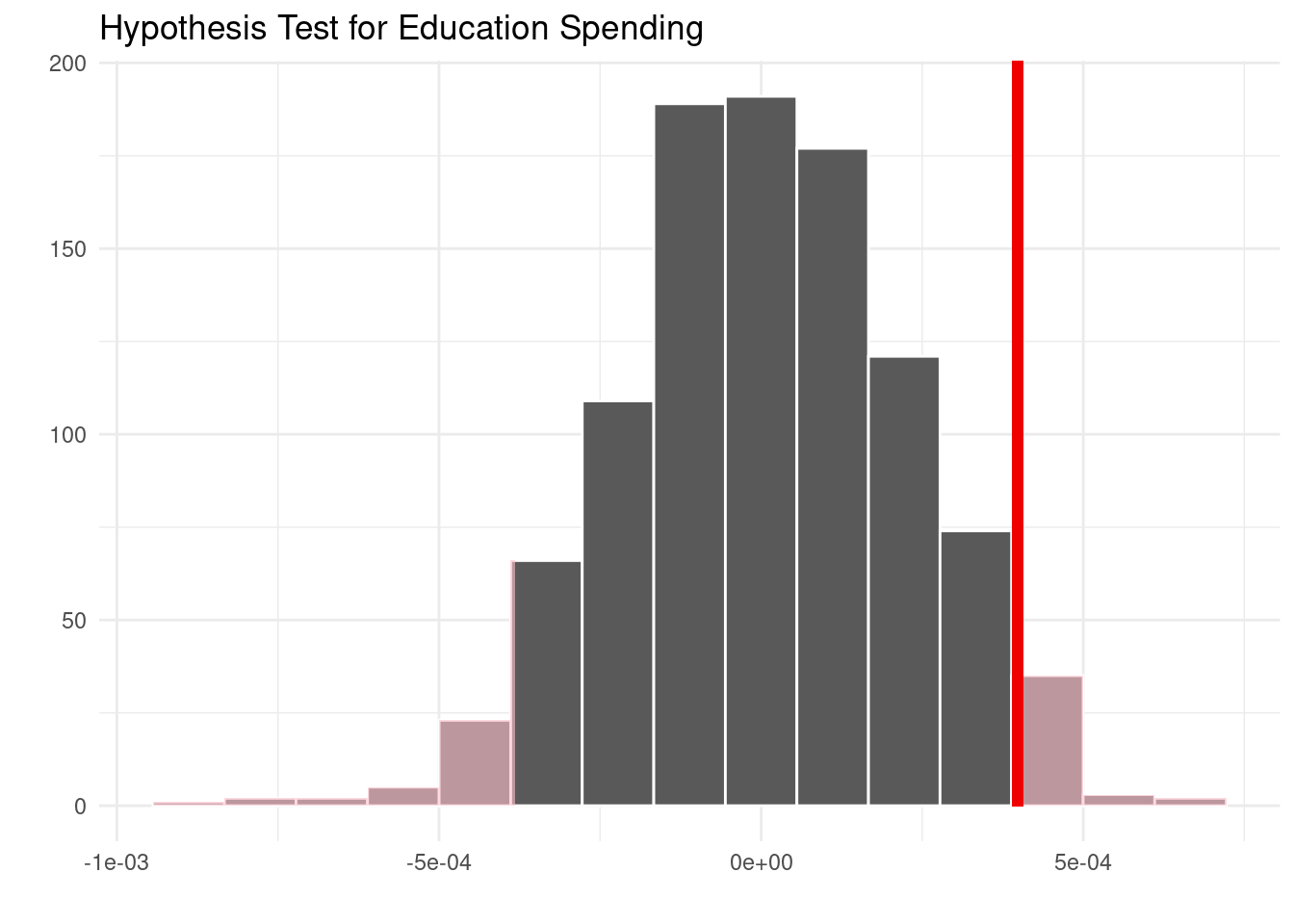
# A tibble: 1 × 1
  p_value
    <dbl>
1   0.072
Since the p-value is 0.072 which is greater than 0.05(95% significance level), we fail to reject the null hypothesis. The data does not provide convincing evidence that the average violence crime rates of states with low per cap education spending and high per cap education spending is different.
Hypothesis Test - Prison
\[ H_0: p_c-p_r=0 \]
\[ H_A: p_c-p_r\neq0 \]
Null Hypothesis: There is no significant difference in violence rate in states with low per cap prison spending and high per cap prison spending.
Alternative Hypothesis: There is a significant difference in violence rate in states with low per cap prison spending and high per cap prison spending.
Warning: The statistic is based on a difference or ratio; by default, for
difference-based statistics, the explanatory variable is subtracted in the
order "high" - "low", or divided in the order "high" / "low" for ratio-based
statistics. To specify this order yourself, supply `order = c("high", "low")` to
the calculate() function.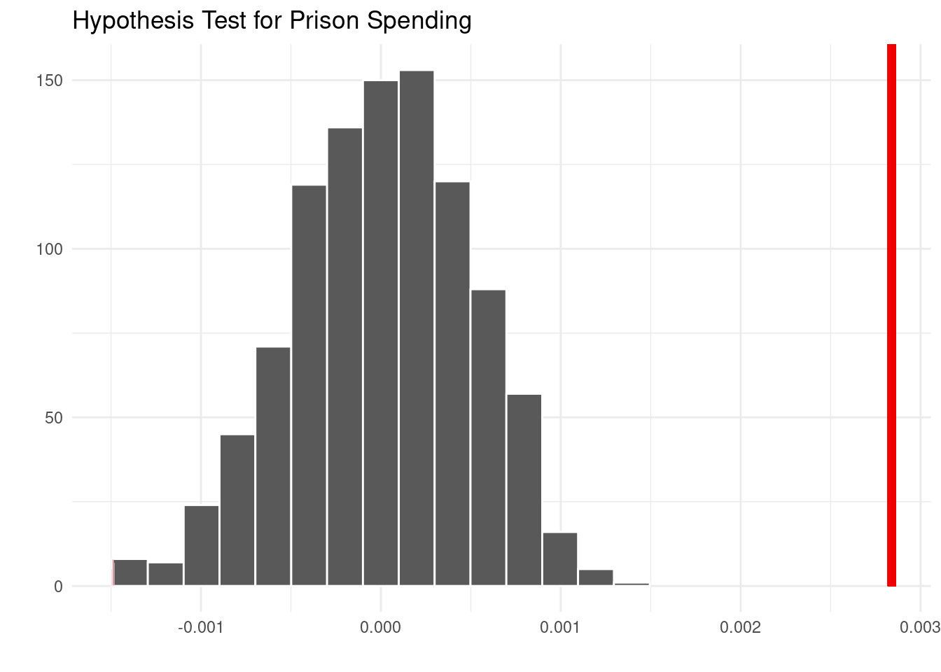
Warning: Please be cautious in reporting a p-value of 0. This result is an
approximation based on the number of `reps` chosen in the `generate()` step. See
`?get_p_value()` for more information.
# A tibble: 1 × 1
p_value
<dbl>
1 0Since the p-value is 0 which is less than any significance level, we can reject the null hypothesis in favor of the alternative hypothesis. The data provides convincing evidence that the average violence crime rates of states with low per cap prison spending and high per cap prison spending is different.
##confidence interval:
\[ \widehat{violence~rate} = 3.635873e^{-03} + 1.827521e^{-10}\times police~spending \]
For every 1 dollar increase in police spending, the predicted violence rate increases by 1.827521e-10, on average.
# A tibble: 2 × 5
  term          estimate std.error statistic  p.value
  <chr>            <dbl>     <dbl>     <dbl>    <dbl>
1 (Intercept)    0.00331  0.000180     18.4  3.46e-48
2 percap_police  0.00655  0.00263       2.50 1.32e- 2
# A tibble: 1 × 2
lower_ci upper_ci
<dbl> <dbl>
1 -1.90e-10 4.78e-10We are 95% confident that for every 1 dollar increase in police spending, the predicted change in violence rate is between -1.899252e-10 and 4.784646e-10, on average.
Interpretation and conclusions
From the data, a few points stick out. Across most of the country, states spend more on education than on police or prisons, per capita. For educational spending per-capita, it is worth noting that Republican states have a higher violence rate compared to other political affiliations. We can also notice the relatively low correlation between different types of spending and violence rates. We can see that this may be because prison and police spending is about the same for each state. New Mexico and Alaska are clear outliers, having higher violence rates than other countries. Nevada has had a major drop in violence rates from 2016 to 2019, although it isn’t clear that it comes from a spending difference.
Limitations
A limitation of our project is that the crime rate data only had data up to 2019. During the peer review session, people commented that having more data, perhaps up until the current year (2023) would have been nice. Still, analyzing data from 50 states proved to be difficult. There was a lot of data to work with, and it was difficult to visualize all of it in a clear and aesthetic manner. Furthermore, although we analyzed data related to spending on police, education, and prisons, it would be nice to relate it to more recent policies regarding crime and spending.