Project title

Appendix to report

Data cleaning

library(ggplot2)
library(readxl)
library(dplyr)

Attaching package: 'dplyr'
The following objects are masked from 'package:stats':

    filter, lag
The following objects are masked from 'package:base':

    intersect, setdiff, setequal, union
library(tidyr)
library(stringr)
library(skimr)
# read in the data
person_data <- read_excel("data/PERSON_DATASET.xlsx")

# Drop unnecessary columns
columns_to_drop <- c("_trust", "_country", "_created_at","_started_at", "_ip", 
                     "1st_choice_gold", "2nd_choice_gold", "_channel",
                     "i_would_not_use_gold","select_your_gender_gold",
                     "select_your_race_gold", "_unit_id", "_tainted", "_id")
person_data_clean <- person_data |>
  select(-one_of(columns_to_drop))

# Rename columns for consistency
column_names <- c("id", "city", "region", "first_choice", "second_choice",
                  "would_not_use", "gender", "race", "image_url")

colnames(person_data_clean) <- column_names

# Step 5: Clean up missing or inconsistent data
person_data_clean <- person_data_clean |>
  mutate(
    gender = recode(gender, "NA" = NA_character_, "I don't know" = "Other"),
    race = recode(race, "NA" = NA_character_),
    target = str_sub(image_url, 12, 17),
    emotion = if_else((str_sub(image_url, 34, 34) == "H"), 
              str_sub(image_url, 34, 35), str_sub(image_url, 34, 34))
    ) 

person_data_clean <- person_data_clean |>
  select(-image_url) 

person_data_clean <- person_data_clean |>
  mutate(
    image_race = case_when(
      str_sub(target, 1, 1) == "A" ~ "Asian",
      str_sub(target, 1, 1) == "B" ~ "Black",
      str_sub(target, 1, 1) == "L" ~ "Latino",
      str_sub(target, 1, 1) == "W" ~ "White"
    ),
    image_gender = case_when(
      str_sub(target, 2, 2) == "M" ~ "Male",
      str_sub(target, 2, 2) == "F" ~ "Female"
    )
  )

# make sure everything is in english and has same capitalization
person_data_clean <- person_data_clean |>
  mutate(
    gender = str_to_lower(gender),
    race = str_to_lower(race)
  ) |>
  mutate(
    gender = case_when(
      gender %in% c("masculino", "male") ~ "male",
      gender %in% c("hembra", "female") ~ "female",
      TRUE ~ "other"
    ),
    race = case_when(
      race %in% c("blanco", "white") ~ "white",
      race %in% c("negro", "black") ~ "black",
      race %in% c("otro", "other") ~ "other",
      TRUE ~ race
    )
  )

person_data_clean <- person_data_clean |>
  mutate(emotion = case_when(
    emotion == "N" ~ "Neutral",
    emotion %in% c("HO", "HC") ~ "Happiness",
    emotion == "A" ~ "Anger",
    emotion == "F" ~ "Fear",
    TRUE ~ emotion))
  
write.csv(person_data_clean, "data/person_data_clean.csv")

person_data_clean
# A tibble: 1,845 × 12
         id city  region   first_choice second_choice would_not_use gender race 
      <dbl> <chr> <chr>    <chr>        <chr>         <chr>         <chr>  <chr>
 1  1856261 FL    Palm Ci… Disgust      Surprise      Happiness     female white
 2 29885393 LA    Lake Ch… Fear         Surprise      Happiness     female white
 3  6432269 OH    Macedon… Sadness      Anger         Happiness     female white
 4  4316379 NY    Bronx    Happiness    Neutral       Anger         female white
 5 45264713 FL    Miami    Happiness    Neutral       Sadness       female lati…
 6  9559045 OK    Jenks    Happiness    Happiness     Anger         female white
 7 44044795 AZ    Lake Ha… Fear         Sadness       Happiness     male   white
 8 27215203 OK    Tulsa    Disgust      Fear          Happiness     female other
 9 44788207 FL    Altamon… Surprise     Fear          Happiness     male   black
10 37243882 IA    Perry    Happiness    Happiness     Anger         male   white
# ℹ 1,835 more rows
# ℹ 4 more variables: target <chr>, emotion <chr>, image_race <chr>,
#   image_gender <chr>
eas_data <- read_excel("data/MICROSOFT_DATASET.xlsx")

eas_data <- eas_data |>
  mutate(
    race = case_when(
      str_sub(Target, 1, 1) == "A" ~ "Asian",
      str_sub(Target, 1, 1) == "B" ~ "Black",
      str_sub(Target, 1, 1) == "L" ~ "Latino",
      str_sub(Target, 1, 1) == "W" ~ "White"
    ),
    gender = case_when(
      str_sub(Target, 2, 2) == "M" ~ "Male",
      str_sub(Target, 2, 2) == "F" ~ "Female"
    )
  )


write.csv(eas_data, "data/eas_data.csv")

eas_data
# A tibble: 1,207 × 12
   Target Emotion SADNESS NEUTRAL CONTEMPT DISGUST ANGER SURPRISE  FEAR
   <chr>  <chr>     <dbl>   <dbl>    <dbl>   <dbl> <dbl>    <dbl> <dbl>
 1 AF-205 N         0       1        0           0     0        0     0
 2 AF-208 N         0       1        0           0     0        0     0
 3 AF-249 N         0.011   0.983    0.005       0     0        0     0
 4 AF-220 N         0.001   0.993    0.001       0     0        0     0
 5 AF-235 N         0.002   0.994    0.003       0     0        0     0
 6 AF-227 N         0       1        0           0     0        0     0
 7 AF-242 N         0.035   0.964    0           0     0        0     0
 8 AF-234 N         0.02    0.979    0.001       0     0        0     0
 9 AF-247 N         0.002   0.954    0.002       0     0        0     0
10 AF-256 N         0.188   0.811    0.001       0     0        0     0
# ℹ 1,197 more rows
# ℹ 3 more variables: HAPPINESS <dbl>, race <chr>, gender <chr>
eas_data_clean <- eas_data |>
  mutate(Emotion = case_when(
    Emotion == "N" ~ "NEUTRAL",
    Emotion %in% c("HO", "HC") ~ "HAPPINESS",
    Emotion == "A" ~ "ANGER",
    Emotion == "F" ~ "FEAR",
    TRUE ~ Emotion
  ))

write.csv(eas_data_clean, "data/eas_data_clean.csv")

eas_data_clean
# A tibble: 1,207 × 12
   Target Emotion SADNESS NEUTRAL CONTEMPT DISGUST ANGER SURPRISE  FEAR
   <chr>  <chr>     <dbl>   <dbl>    <dbl>   <dbl> <dbl>    <dbl> <dbl>
 1 AF-205 NEUTRAL   0       1        0           0     0        0     0
 2 AF-208 NEUTRAL   0       1        0           0     0        0     0
 3 AF-249 NEUTRAL   0.011   0.983    0.005       0     0        0     0
 4 AF-220 NEUTRAL   0.001   0.993    0.001       0     0        0     0
 5 AF-235 NEUTRAL   0.002   0.994    0.003       0     0        0     0
 6 AF-227 NEUTRAL   0       1        0           0     0        0     0
 7 AF-242 NEUTRAL   0.035   0.964    0           0     0        0     0
 8 AF-234 NEUTRAL   0.02    0.979    0.001       0     0        0     0
 9 AF-247 NEUTRAL   0.002   0.954    0.002       0     0        0     0
10 AF-256 NEUTRAL   0.188   0.811    0.001       0     0        0     0
# ℹ 1,197 more rows
# ℹ 3 more variables: HAPPINESS <dbl>, race <chr>, gender <chr>
choice_correct_eas <- eas_data_clean |>
  rowwise() |>
  mutate(
    value = max(c_across(SADNESS:HAPPINESS)),
     PredictedEmotion = names(eas_data_clean)
      [which.max(c_across(SADNESS:HAPPINESS)) + 2]             
    ) |>
  select(-SADNESS:-value) |>
  mutate(Correct = Emotion == PredictedEmotion)


write.csv(choice_correct_eas, "data/choice_correct_eas.csv")

Other appendicies (as necessary)

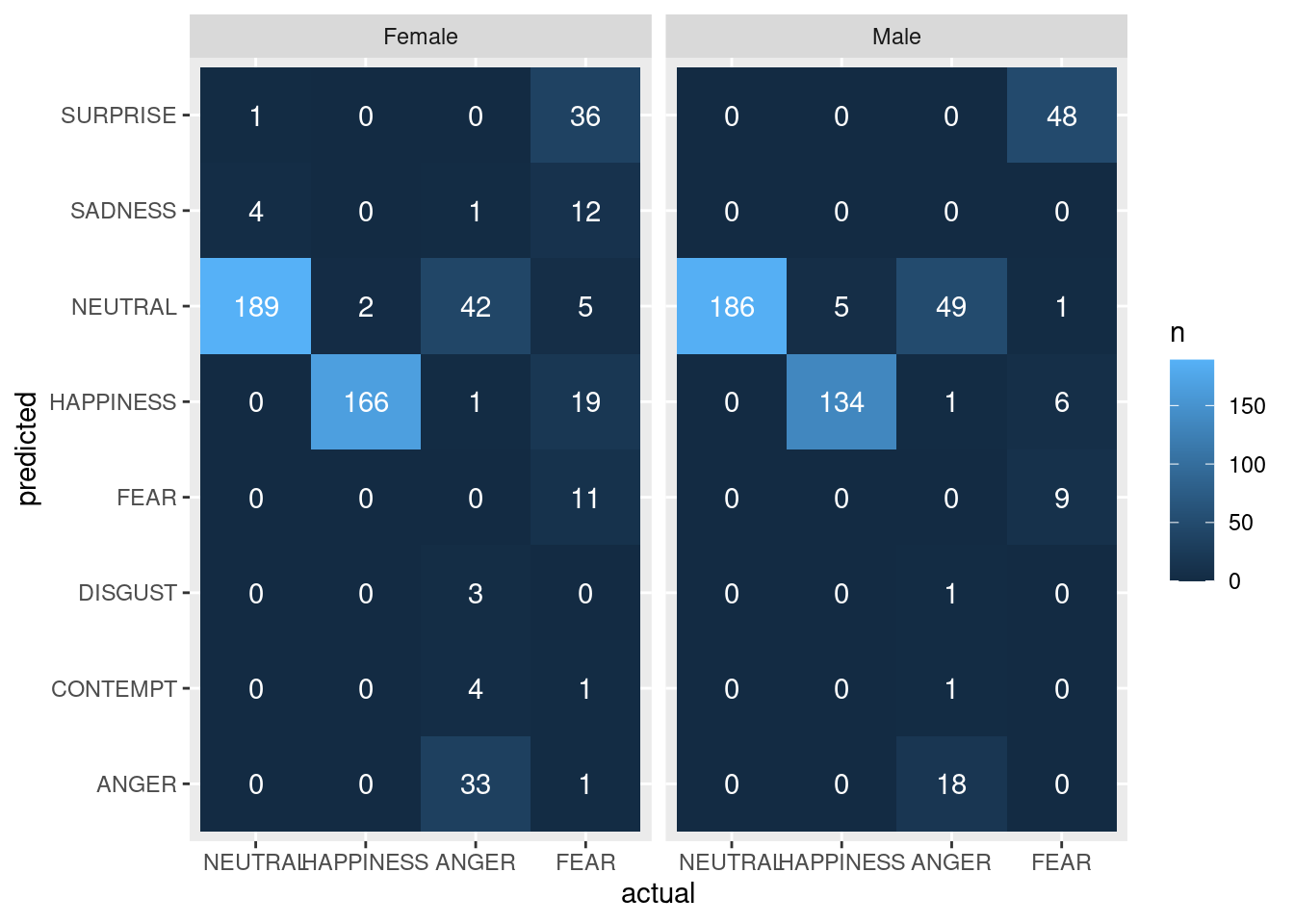
These code chunks show the results from analyzing gender and exploring if there is any gender bias. Interestingly, the pvalues showed that there is a significant difference in the guessing accuracy for the emotion “fear” in females compared to males(pvalue = 0.00085). Fear is often confused with surprise and happinessin females. Although these findings are interesting, they are not very relevant to our study.

probs <- eas_data |>
  select(SADNESS:HAPPINESS)

preds <- colnames(probs)[apply(probs, 1, which.max)]

df <- eas_data |>
  mutate(actual = factor(Emotion, levels= c("N" , "HC" ,"A",  "HO" ,"F" ), 
                          labels=c('NEUTRAL', 'HAPPINESS', 'ANGER', 'HAPPINESS', 'FEAR'))) |>
  mutate(predicted = preds) |>
  mutate(accuracy = predicted == actual ) 

df |>
  filter(race %in% c('Black', 'White')) |>
  count(gender, predicted, actual) |>
  complete(predicted, actual, gender, fill=list(n=0)) |>
  ggplot(aes(x=actual, y=predicted, fill=n)) + geom_tile() + facet_wrap(~gender) +
  geom_text(aes(label=n), color='white')

res <- data.frame()
for (cat in unique(df$actual)){
  cur <- df |>
    filter(actual == cat, race %in% c('Black', 'White'))
  comp <- chisq.test(table(cur$gender, cur$predicted))
  res <- bind_rows(res, data.frame(category=cat, statisitcs=comp$statistic, pvalue=comp$p.value))
}
Warning in chisq.test(table(cur$gender, cur$predicted)): Chi-squared
approximation may be incorrect

Warning in chisq.test(table(cur$gender, cur$predicted)): Chi-squared
approximation may be incorrect

Warning in chisq.test(table(cur$gender, cur$predicted)): Chi-squared
approximation may be incorrect

Warning in chisq.test(table(cur$gender, cur$predicted)): Chi-squared
approximation may be incorrect
res <- res |>
  tibble::rownames_to_column() |> 
  select(-rowname)
res
   category statisitcs       pvalue
1   NEUTRAL   4.857732 0.0881367248
2 HAPPINESS   1.044670 0.3067378368
3     ANGER   7.539811 0.1834877455
4      FEAR  22.834811 0.0008537349