Substance Use, Abuse, and the Impact of Age on Patterns and Behaviors
Introduction
As recreational drug use becomes more prevalent and accepted in the United States, particularly in the case of recreational Cannabis use, it is important to understand the broader trends and potentially broad implications those trends have on society. This report is a relatively small contribution to the wider body of knowledge concerning drug use in the United States that seeks to understand the relationships between age and substance use and abuse. We wanted to understand whether age was a contributing factor to whether individuals abused substances and if whether it could inform individuals choice in the substance they used from some of the most popular recreational drugs: alcohol, cannabis, tobacco, and cocaine.
Using widely available data from the National Survey on Drug Use and Health we looked at the summary statistics for the rates of use and abuse of a particular substance for a given age category and formulated a null-hypothesis significance to evaluate whether age played a significant role in drug abuse and “drug of choice”. We were curious as to whether individuals, especially adolescents, tended towards one substance or another and whether that changed overtime with age. We find this question especially pressing as legalization efforts accross the United States for substances such as Cannabis, which is shown to have certain medical uses, have increased the amount of discourse about the implications of legalization/acceptance of certain substances. As for our question of age’s role, in abuse we wondered whether the potential of increased ease of access as a result of legalization could lead younger individuals to consume substance they might not have otherwise.
Our findings below suggest that it is unlikely that age is the determining factor in substance abuse, although it does not rule out the role of age entirely. To be more specific, the results indicate the use rate for marijuana is higher in states with medical, decriminalized, or recreational legalization compared to states with illegal status for the 18-25 age group. However, it is important to note that this association is not uniform across all age groups, with the 12-17 age group showing a less pronounced increase in use rate due to legalization.
Data description
Motivation:
The Drugs data set from CORGIS was compiled by the CORGIS to be used as open source data in analysis by whoever wanted to use it. It was compiled from data from the National Survey on Drug Use and Health (NSDUH), which is administered by the Substance Abuse and Mental Health Administration (SAMHSA) to “provide estimates of substance use and mental illness at the national, state, and sub-state levels” and “help identify the extent of substance use and mental illness among different subgroups, estimate trends over time, and determine the need for treatment services” to “allow researchers, clinicians, policymakers, and the general public to better understand and improve the nation’s behavioral health”. The data collection is publicly funded through the U.S. Department of Health and Human Services.
The State Marijuana Laws (2019) data set was compiled by Selene Arrazolo in 2016 as a personal project for data.world from data collected by Michael Maciag funded by Governing Data, a magazine based in Washington, D.C. that covers state and local government that is owned by e.Republic a Folsom, California-based research and media company that focuses on connecting private IT companies with government and education agencies and maintains multiple publications, platforms, and brands all concerned with technology and government. The data set was updated to reflect the legal status of marijuana by state in 2019 and include decriminalization as a variable.
Composition:
The drugs data set is comprised of summary functions of the survey data collected by SAMHSA through the NSDUH from 2002-2019. The data represents the responses of individuals collected in face-to-face household interviews in all 50 states and the District of Columbia. The survey it was collected through covers residents of households, persons in non-institutional group quarters, and civilians living on military bases. It excludes individuals experiencing homelessness who do not use shelters, active military personnel, and residents of institutional group quarters such as jails, nursing homes, mental institutions, and long-term care hospitals. The original SAMHSA data sets identified five subgroups by residence state and an exhaustive list of different substances. The data set compiled by CORGIS combined the five original age groups to form three, and only includes alcohol, cigarette, tobacco, marijuana, and cocaine use.
The State Marijuana Laws (2019) data set is comprised of boolean variables relating to the legal status of marijuana in all 50 states and the District of Columbia. It was collected through research of publicly available data.
Collection:
The drugs data set is a compilation of data collected through the NSDUH from 2002-2019. The survey is a face-to-face interview by trained interviewing staff managed by field supervisors who, in turn, reported to regional supervisors. The interviewing staff was trained and use a questionnaire written by SAMHSA to conduct the interviews. Starting in 2018 respondents were offered a $30 incentive which had the expected effect of increasing the response rate. Interviewing staff were trained on the ethics and regulations involving research on human subjects.
The State Marijuana Laws (2019) data set was collected from publicly available records on state laws and public information on the internet.
Processing/cleaning/labeling:
The raw data collected through the NSDUH was processed into summary statistics by SAMHSA, but CORGIS compiled the data set from the raw data from NSDUH. It includes both totals (in thousands of people) and rates (as a percentage of the population) for each age subgroup compiled, 12-17, 18-25, and 26+, as well as the related states each respondent resided in when the data was collected. The data set is made up of data collected annually through the NSDUH from 2002-2019.
The State Marijuana Laws (2019) data set is unprocessed and only links the legal status of marijuana in 2019 in each state to its respective row.
Uses:
All of the data used in this project has likely been used before in other analyses as all the data is publicly available. The State Marijuana Laws (2019) data set was created for the use of this project only but was compiled from existing publicly available information. All the raw data for the drugs data set is available on the SAMHSA website, and the raw data for the State Marijuana Laws (2019) data set is available on Wikipedia.
Data analysis
Research Question: Are individuals more likely to abuse one substance over another based on their age?
Loading required package: Matrix

Attaching package: 'Matrix'

The following objects are masked from 'package:tidyr':

    expand, pack, unpack

Loaded glmnet 4.1-7
# subset for rate of alcohol use disorder in past yearalcohol_year_rate <- drugUse[, c("Rates.Alcohol.Use.Disorder.Past.Year.12.17", "Rates.Alcohol.Use.Disorder.Past.Year.18.25", "Rates.Alcohol.Use.Disorder.Past.Year.26.")]# subset for rate of ilicit drug use in past yearilicit_year_rate <- drugUse[, c("Rates.Illicit.Drugs.Cocaine.Used.Past.Year.12.17", "Rates.Illicit.Drugs.Cocaine.Used.Past.Year.18.25", "Rates.Illicit.Drugs.Cocaine.Used.Past.Year.26.")]# subset for rate of marijuana use in past yearmarijuana_year_rate <- drugUse[, c("Rates.Marijuana.Used.Past.Year.12.17", "Rates.Marijuana.Used.Past.Year.18.25", "Rates.Marijuana.Used.Past.Year.26.")]# alc mean and sdalcohol_year_rate_mean <-c(mean(drugUse$Rates.Alcohol.Use.Disorder.Past.Year.12.17), mean(drugUse$Rates.Alcohol.Use.Disorder.Past.Year.18.25), mean(drugUse$Rates.Alcohol.Use.Disorder.Past.Year.26.))alcohol_year_rate_sd <-c(sd(drugUse$Rates.Alcohol.Use.Disorder.Past.Year.12.17), sd(drugUse$Rates.Alcohol.Use.Disorder.Past.Year.18.25), sd(drugUse$Rates.Alcohol.Use.Disorder.Past.Year.26.))alcohol_summary <-data.frame(age_group =c("12-17", "18-25", "26+"),mean = alcohol_year_rate_mean,sd = alcohol_year_rate_sd)# illicit mean and sdilicit_year_rate_mean <-c(mean(drugUse$Rates.Illicit.Drugs.Cocaine.Used.Past.Year.12.17), mean(drugUse$Rates.Illicit.Drugs.Cocaine.Used.Past.Year.18.25), mean(drugUse$Rates.Illicit.Drugs.Cocaine.Used.Past.Year.26.))ilicit_year_rate_sd <-c(sd(drugUse$Rates.Illicit.Drugs.Cocaine.Used.Past.Year.12.17), sd(drugUse$Rates.Illicit.Drugs.Cocaine.Used.Past.Year.18.25), sd(drugUse$Rates.Illicit.Drugs.Cocaine.Used.Past.Year.26.))ilicit_summary <-data.frame(age_group =c("12-17", "18-25", "26+"),mean = ilicit_year_rate_mean,sd = ilicit_year_rate_sd)# marijuana mean and sdmarijuana_year_rate_mean <-c(mean(drugUse$Rates.Marijuana.Used.Past.Year.12.17), mean(drugUse$Rates.Marijuana.Used.Past.Year.18.25), mean(drugUse$Rates.Marijuana.Used.Past.Year.26.))marijuana_year_rate_sd <-c(sd(drugUse$Rates.Marijuana.Used.Past.Year.12.17), sd(drugUse$Rates.Marijuana.Used.Past.Year.18.25), sd(drugUse$Rates.Marijuana.Used.Past.Year.26.))marijuana_summary <-data.frame(age_group =c("12-17", "18-25", "26+"),mean = marijuana_year_rate_mean,sd = marijuana_year_rate_sd)# summary tablesalcohol_summary
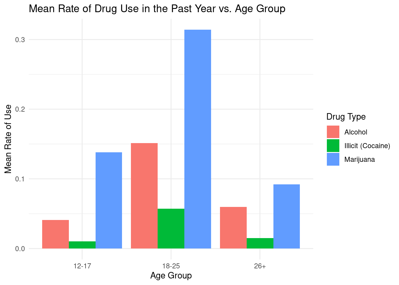
# combine data into one dfsummary_total_data <-rbind(transform(alcohol_summary, drug_type ="Alcohol"),transform(ilicit_summary, drug_type ="Illicit (Cocaine)"),transform(marijuana_summary, drug_type ="Marijuana"))# create histogramggplot(summary_total_data, aes(x = age_group, y = mean, fill = drug_type)) +geom_bar(position ="dodge", stat ="identity") +# change color and themescale_color_colorblind() +theme_minimal() +# add labelslabs(title ="Mean Rate of Drug Use in the Past Year vs. Age Group",x ="Age Group",y ="Mean Rate of Use",fill ="Drug Type")
This visualization shows the mean rate of drug use in the past year divided into 3 age groups (12-17, 18-25, 26+) Focus on 3 types of drugs: Alcohol, Illicit Drugs (Cocaine), and Marijuana. The visualization shows that age groups 18-25 have the overall highest mean rate of drugs used for all 3 categories in the past year.
rate_columns <-c("Year", "State", "Rates.Alcohol.Use.Past.Month.12.17", "Rates.Alcohol.Use.Past.Month.18.25", "Rates.Alcohol.Use.Past.Month.26.","Rates.Tobacco.Use.Past.Month.12.17","Rates.Tobacco.Use.Past.Month.18.25","Rates.Tobacco.Use.Past.Month.26.","Rates.Marijuana.Used.Past.Month.12.17", "Rates.Marijuana.Used.Past.Month.18.25", "Rates.Marijuana.Used.Past.Month.26.","Rates.Illicit.Drugs.Cocaine.Used.Past.Year.12.17", "Rates.Illicit.Drugs.Cocaine.Used.Past.Year.18.25", "Rates.Illicit.Drugs.Cocaine.Used.Past.Year.26.")drugUse_pastMonthRates_sub <- drugUse[, rate_columns]# reshape the data to long formatlong_drugUse <- drugUse_pastMonthRates_sub |>pivot_longer(cols =starts_with("Rates"),names_to =c("Substance", "Age.Group"),names_pattern ="Rates\\.(.*)\\.Past\\.Year\\.(.*)",values_to ="Rate") |>mutate(Substance =str_extract(Substance, "Alcohol|Marijuana|Cocaine"))# convert Age.Group numeric values to factorslong_drugUse$Age.Group <-factor(long_drugUse$Age.Group, levels =c("12.17", "18.25", "26."), labels =c("12-17", "18-25", "26+"))
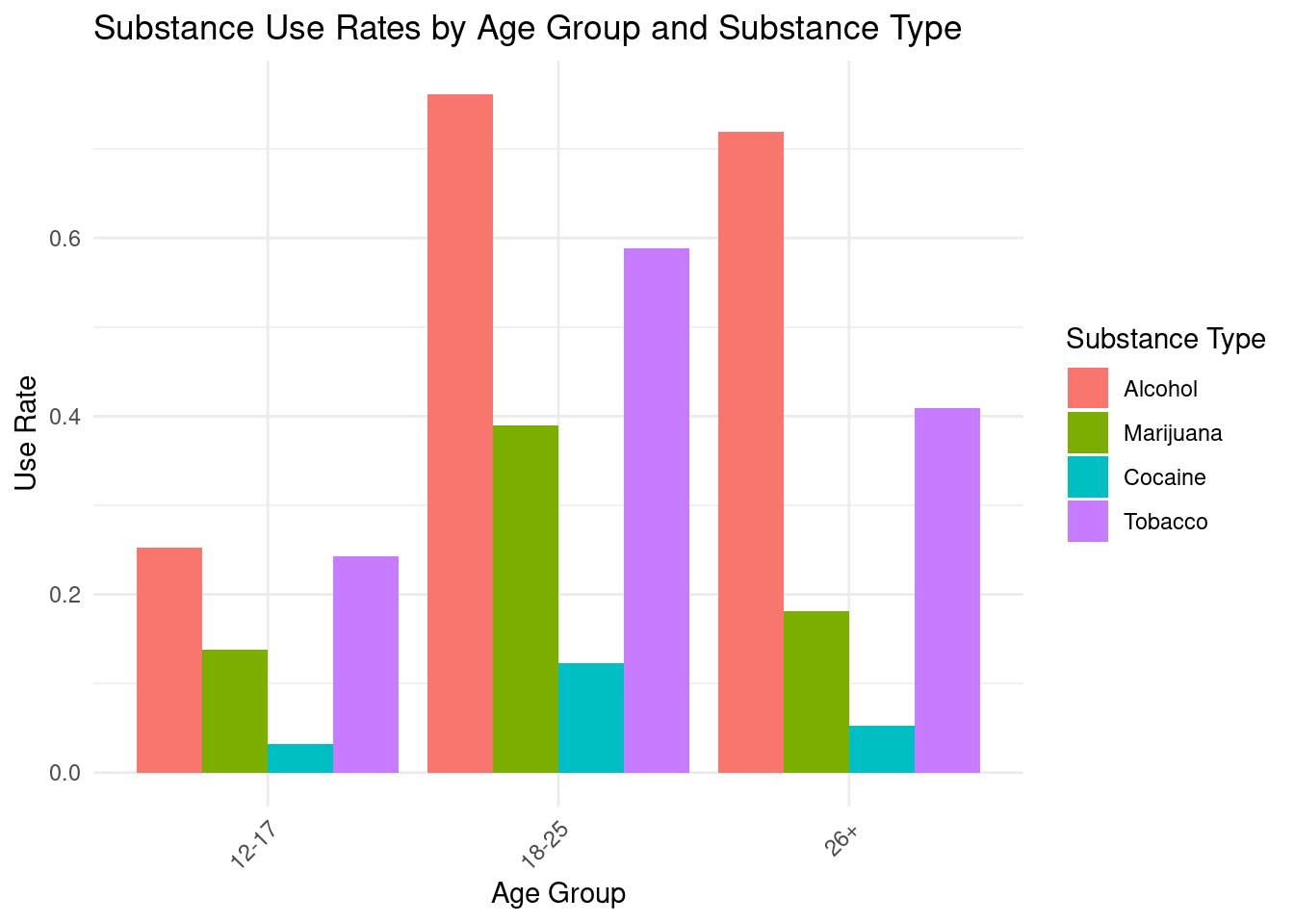
#pivot data to create Substance Type and Age Group columns and factor those columnsdrugUse_long_factored <- drugUse_pastMonthRates_sub |>pivot_longer(cols =starts_with("Rates."),names_to =c("Substance Type", "Age Group"),names_pattern ="(?:Rates|Rates.Illicit.Drugs)\\.([a-zA-Z ]*)\\.(?:Use|Used)\\.Past\\.(?:Month|Year)\\.(..*)?",values_to ="Use Rate") |>mutate( `Age Group`=factor(`Age Group`,levels =c("12.17", "18.25", "26."),labels =c("12-17", "18-25", "26+")),`Substance Type`=factor(`Substance Type`,levels =c("Alcohol", "Marijuana", "Cocaine", "Tobacco"),labels =c("Alcohol", "Marijuana", "Cocaine", "Tobacco")))
#create grouped bar plotdrugUse_grouped_bar <-ggplot(data = drugUse_long_factored, aes(x =`Age Group`, y =`Use Rate`, fill =`Substance Type`)) +geom_bar(stat ="identity", position ="dodge") +theme_minimal() +labs(title ="Substance Use Rates by Age Group and Substance Type",x ="Age Group",y ="Use Rate",fill ="Substance Type") +theme(axis.text.x =element_text(angle =45, hjust =1))drugUse_grouped_bar
# calculate the max rate to adjust y axis accordinglymax_sum_rate <- long_drugUse |>group_by(Year, Substance) |>summarize(total_rate =sum(Rate)) |>ungroup() |>summarize(max_sum_rate =max(total_rate)) |>pull(max_sum_rate)
`summarise()` has grouped output by 'Year'. You can override using the
`.groups` argument.
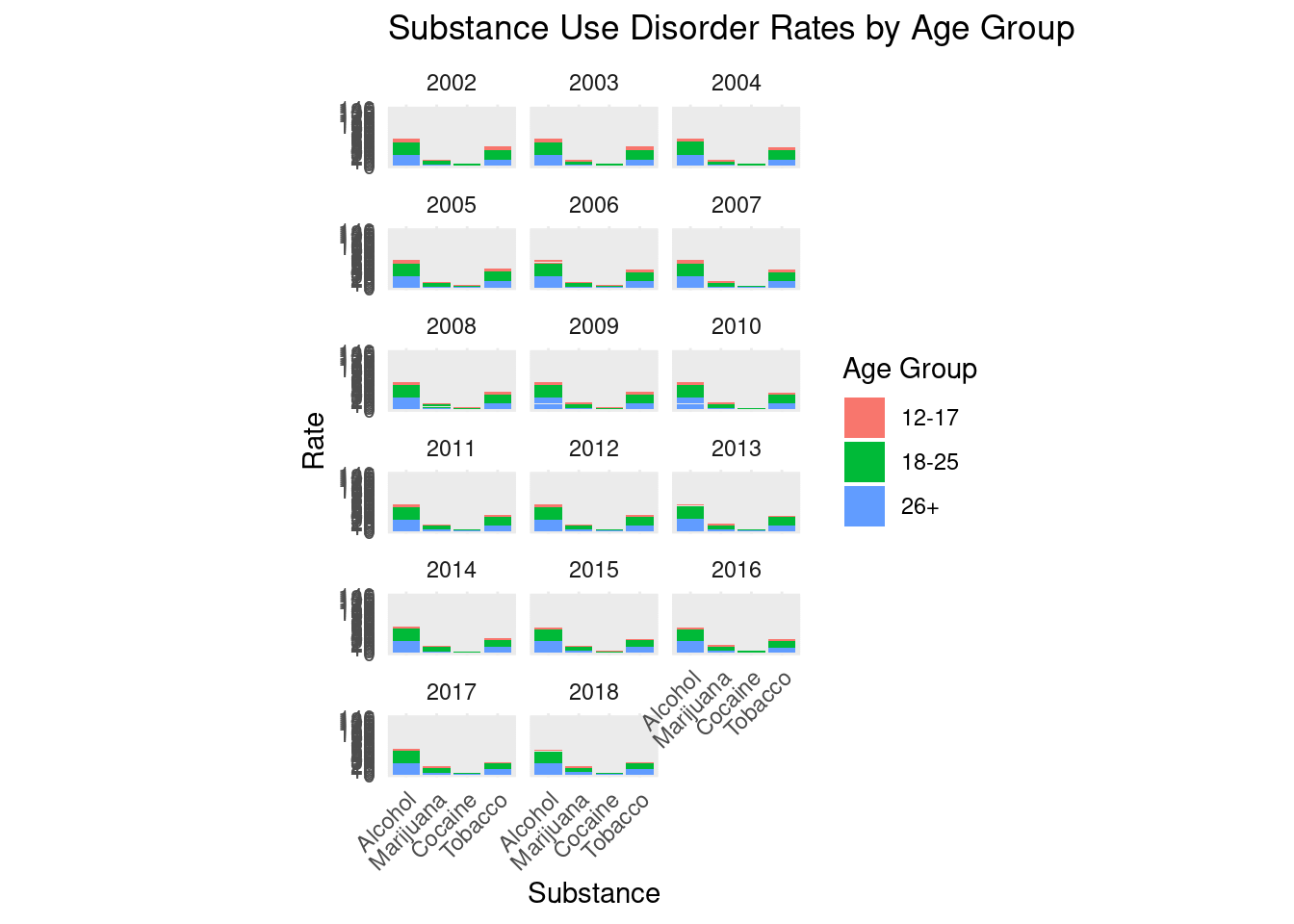
# create faceted bar plotfaceted_rates_plot <-ggplot(drugUse_long_factored, aes(x =`Substance Type`, y =`Use Rate`, fill =`Age Group`)) +geom_bar(stat ="identity", position ="stack") +facet_wrap(~ Year, ncol =3) +labs(title ="Substance Use Disorder Rates by Age Group",x ="Substance",y ="Rate") +theme_minimal() +theme(axis.text.x =element_text(angle =45, hjust =1),strip.background =element_blank(),aspect.ratio = .5) +scale_y_continuous(limits =c(0, max_sum_rate *1.1), breaks =seq(0, max_sum_rate *1.1, by =5))faceted_rates_plot
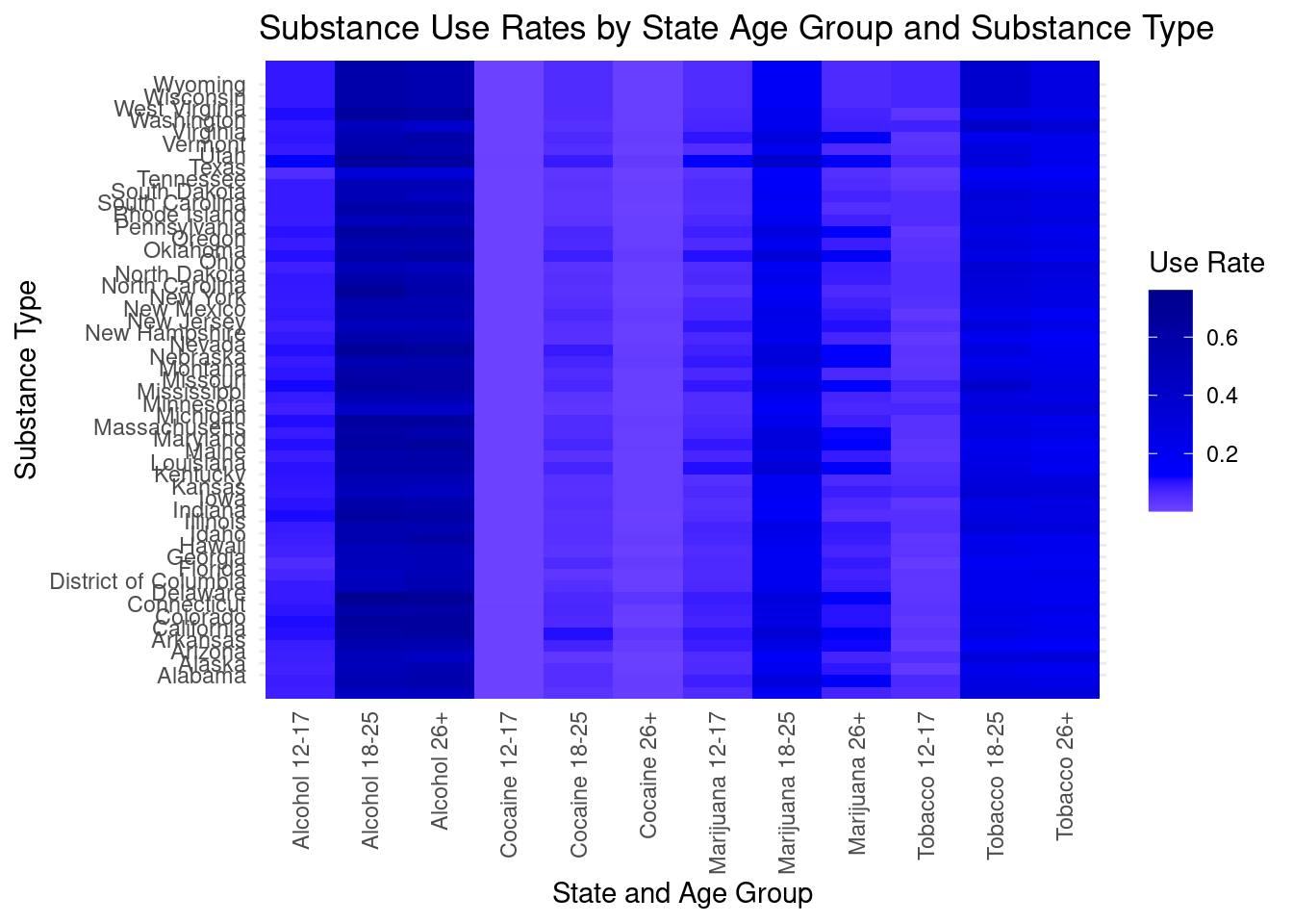
#mutate drugUse_long_factored to add a new column that combines the state and age group variablesdrugUse_heatmap_sub <- drugUse_long_factored |>mutate(`Substance AgeGroup`=paste(`Substance Type`,`Age Group`, sep =" "))#create a heatmap where each square represents the use rate or each age group in each statedrugUse_heatmap <-ggplot(data = drugUse_heatmap_sub, aes(x =`Substance AgeGroup`, y = State, fill =`Use Rate`)) +geom_tile(height =4) +scale_fill_gradient2(low ="white", mid ="blue", high ="darkblue", midpoint =median(drugUse_heatmap_sub$`Use Rate`)) +theme_minimal() +labs(title ="Substance Use Rates by State Age Group and Substance Type",x ="State and Age Group",y ="Substance Type",fill ="Use Rate") +theme(axis.text.x =element_text(angle =90, hjust =1, vjust =0.5))drugUse_heatmap
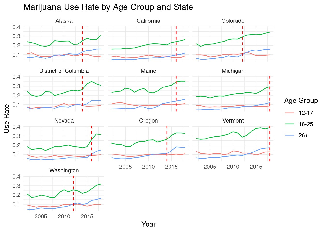
#join drugUse and legalStatusdrugUse_legalStatus_joined <- drugUse_long_factored |>left_join(legalStatus, by =c("Year", "State")) |>filter(`Substance Type`=="Marijuana", Legalization_Year !=2020)
#create the faceted line plot with the use rate of marijuana #for each age group as a line and the facets as the statesggplot(drugUse_legalStatus_joined, aes(x = Year, y =`Use Rate`, color =`Age Group`)) +geom_line() +facet_wrap(~ State, ncol =3) +geom_vline(data =subset( drugUse_legalStatus_joined, !is.na(Legalization_Year)), aes(xintercept = Legalization_Year), color ="red", linetype ="dashed") +labs(title ="Marijuana Use Rate by Age Group and State",x ="Year",y ="Use Rate",color ="Age Group") +theme_minimal()
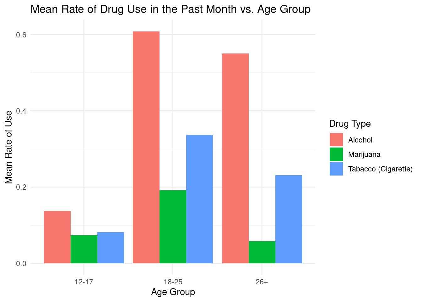
# subset for rate of alcohol use disorder in past monthalcohol_month_rate <- drugUse[, c("Rates.Alcohol.Use.Past.Month.12.17", "Rates.Alcohol.Use.Past.Month.18.25", "Rates.Alcohol.Use.Past.Month.26.")]# subset for rate of tabacco use disorder in past monthtobacco_month_rate <- drugUse[, c("Rates.Tobacco.Cigarette.Past.Month.12.17", "Rates.Tobacco.Cigarette.Past.Month.18.25", "Rates.Tobacco.Cigarette.Past.Month.26.")]# subset for rate of marijuana use in past monthmarijuana_month_rate <- drugUse[, c("Rates.Marijuana.Used.Past.Month.12.17", "Rates.Marijuana.Used.Past.Month.18.25", "Rates.Marijuana.Used.Past.Month.26.")]# alcohol mean and sdalcohol_month_rate_mean <-c(mean(drugUse$Rates.Alcohol.Use.Past.Month.12.17), mean(drugUse$Rates.Alcohol.Use.Past.Month.18.25), mean(drugUse$Rates.Alcohol.Use.Past.Month.26.))alcohol_month_rate_sd <-c(sd(drugUse$Rates.Alcohol.Use.Past.Month.12.17), sd(drugUse$Rates.Alcohol.Use.Past.Month.18.25), sd(drugUse$Rates.Alcohol.Use.Past.Month.26.))alcohol_summary <-data.frame(age_group =c("12-17", "18-25", "26+"),mean = alcohol_month_rate_mean,sd = alcohol_month_rate_sd)# tobacco mean and sdtobacco_month_rate_mean <-c(mean(drugUse$Rates.Tobacco.Cigarette.Past.Month.12.17), mean(drugUse$Rates.Tobacco.Cigarette.Past.Month.18.25), mean(drugUse$Rates.Tobacco.Cigarette.Past.Month.26.))tobacco_month_rate_sd <-c(sd(drugUse$Rates.Tobacco.Cigarette.Past.Month.12.17), sd(drugUse$Rates.Tobacco.Cigarette.Past.Month.18.25), sd(drugUse$Rates.Tobacco.Cigarette.Past.Month.26.))tobacco_summary <-data.frame(age_group =c("12-17", "18-25", "26+"),mean = tobacco_month_rate_mean,sd = tobacco_month_rate_sd)# marijuana mean and sdmarijuana_month_rate_mean <-c(mean(drugUse$Rates.Marijuana.Used.Past.Month.12.17), mean(drugUse$Rates.Marijuana.Used.Past.Month.18.25), mean(drugUse$Rates.Marijuana.Used.Past.Month.26.))marijuana_month_rate_sd <-c(sd(drugUse$Rates.Marijuana.Used.Past.Month.12.17), sd(drugUse$Rates.Marijuana.Used.Past.Month.18.25), sd(drugUse$Rates.Marijuana.Used.Past.Month.26.))marijuana_summary <-data.frame(age_group =c("12-17", "18-25", "26+"),mean = marijuana_month_rate_mean,sd = marijuana_month_rate_sd)# combine data into one dfsummary_total_data <-rbind(transform(alcohol_summary, drug_type ="Alcohol"),transform(tobacco_summary, drug_type ="Tabacco (Cigarette)"),transform(marijuana_summary, drug_type ="Marijuana"))# create histogramggplot(summary_total_data, aes(x = age_group, y = mean, fill = drug_type)) +geom_bar(position ="dodge", stat ="identity") +# change color and themescale_color_colorblind() +theme_minimal() +# add labelslabs(title ="Mean Rate of Drug Use in the Past Month vs. Age Group",x ="Age Group",y ="Mean Rate of Use",fill ="Drug Type")
This visualization shows the mean rate of drug use in the past month divided into 3 age groups (12-17, 18-25, 26+) Focus on 3 types of drugs: Alcohol, Tobacco (Cigarettes), and Marijuana. Similar to the previous visualization, we can clearly see that age groups 18-25 have the overall highest mean rate of drugs used for all 3 categories in the past month.
Evaluation of significance
Null Hypothesis: There is no difference in the means of substance use rates across age groups.
In the equation, ρ is the population correlation coefficient between age and the likelihood of abusing one substance over another.
\[
H_0: p = 0
\]
Alternative Hypothesis: There is a significant relationship between age and the likelihood of abusing one substance over another.
# filter the data frame for the substance typesubstance_type <-"Alcohol"filtered_data <- drugUse_long_factored |>filter(`Substance Type`== substance_type)# perform the ANOVA testanova_result <-aov(`Use Rate`~`Age Group`, data = filtered_data)# check the ANOVA resultssummary(anova_result)
              Df Sum Sq Mean Sq F value Pr(>F)
`Age Group`    2 114.65   57.32   12550 <2e-16 ***
Residuals   2598  11.87    0.00
---
Signif. codes:  0 '***' 0.001 '**' 0.01 '*' 0.05 '.' 0.1 ' ' 1
# filter the data frame for the substance typesubstance_type <-"Tobacco"filtered_data <- drugUse_long_factored |>filter(`Substance Type`== substance_type)# perform the ANOVA testanova_result <-aov(`Use Rate`~`Age Group`, data = filtered_data)# check the ANOVA resultssummary(anova_result)
              Df Sum Sq Mean Sq F value Pr(>F)
`Age Group`    2  38.49  19.244    5602 <2e-16 ***
Residuals   2598   8.92   0.003
---
Signif. codes:  0 '***' 0.001 '**' 0.01 '*' 0.05 '.' 0.1 ' ' 1
# filter the data frame for the substance typesubstance_type <-"Marijuana"filtered_data <- drugUse_long_factored |>filter(`Substance Type`== substance_type)# perform the ANOVA testanova_result <-aov(`Use Rate`~`Age Group`, data = filtered_data)# check the ANOVA resultssummary(anova_result)
              Df Sum Sq Mean Sq F value Pr(>F)
`Age Group`    2  9.315   4.657    3560 <2e-16 ***
Residuals   2598  3.398   0.001
---
Signif. codes:  0 '***' 0.001 '**' 0.01 '*' 0.05 '.' 0.1 ' ' 1
# filter the data frame for the substance typesubstance_type <-"Cocaine"filtered_data <- drugUse_long_factored |>filter(`Substance Type`== substance_type)# perform the ANOVA testanova_result <-aov(`Use Rate`~`Age Group`, data = filtered_data)# check the ANOVA resultssummary(anova_result)
              Df Sum Sq Mean Sq F value Pr(>F)
`Age Group`    2 1.1438  0.5719    4432 <2e-16 ***
Residuals   2598 0.3353  0.0001
---
Signif. codes:  0 '***' 0.001 '**' 0.01 '*' 0.05 '.' 0.1 ' ' 1
#join drugUse and legalStatus create a binary variable for recreational legal statusdrugUse_legalStatus_joined <- drugUse_long_factored |>left_join(legalStatus, by =c("Year", "State")) #filter for adolescents and marijuanafiltered_drugUse_legalStatus_joined <- drugUse_legalStatus_joined |>filter(`Age Group`=="12-17", `Substance Type`=="Marijuana")#create binary for pre legalization years and post legalization yearsfiltered_drugUse_legalStatus_joined$Legal <-ifelse( filtered_drugUse_legalStatus_joined$Year >= filtered_drugUse_legalStatus_joined$Legalization_Year, 1, 0)
Each analysis resulted in a p-value of less than 2e-16, essentially zero. This implies a significant difference in use rate across age groups means that the average use rates of a given substance type are not the same for all age groups. In other words, the proportion of people using a specific substance within one age group is significantly different from the proportion of people using the same substance within another age group.
This finding implies that age is an important factor in the use of a particular substance type. It suggests that substance use behavior might be influenced by factors that vary across different age groups, such as social environment, peer influence, availability, or developmental stage.
We ran a second analysis using a linear regression model to try and determine whether the effects of legalization increased use rate and if this increase was uniform across age groups. The main effect coefficients for Legal_StatusMedical, Legal_StatusDecriminalized, and Legal_StatusRecreational show the differences in use rate for the 18-25 age group compared to the reference category (illegal status) when the age group is held constant. All these coefficients are positive, which indicates that the use rate for marijuana is higher in states with medical, decriminalized, or recreational legalization compared to states with illegal status for the 18-25 age group.
The difference in use rate between medical legalization and illegal status for the 12-17 age group is 0.041704 units lower than the difference for the 18-25 age group. This means that the effect of medical legalization on use rate is less pronounced for the 12-17 age group compared to the 18-25 age group.
The difference in use rate between decriminalized status and illegal status for the 12-17 age group is 0.010512 units lower than the difference for the 18-25 age group. This implies that the effect of decriminalized status on use rate is also less pronounced for the 12-17 age group compared to the 18-25 age group.
The difference in use rate between recreational legalization and illegal status for the 12-17 age group is 0.103296 units lower than the difference for the 18-25 age group. This indicates that the effect of recreational legalization on use rate is less pronounced for the 12-17 age group compared to the 18-25 age group.
The difference in use rate between medical legalization and illegal status for the 26+ age group is 0.028477 units lower than the difference for the 18-25 age group. This means that the effect of medical legalization on use rate is less pronounced for the 26+ age group compared to the 18-25 age group.
The difference in use rate between decriminalized status and illegal status for the 26+ age group is 0.009111 units lower than the difference for the 18-25 age group. This implies that the effect of decriminalized status on use rate is also less pronounced for the 26+ age group compared to the 18-25 age group.
The difference in use rate between recreational legalization and illegal status for the 26+ age group is 0.038879 units lower than the difference for the 18-25 age group. This indicates that the effect of recreational legalization on use rate is less pronounced for the 26+ age group compared to the 18-25 age group.
These interaction terms suggest that the effect of legalization on use rate is not the same across different age groups. For both the 12-17 age group and the 26+ age group, the effect of legalization (be it medical, decriminalized, or recreational) on use rate appears to be less pronounced compared to the 18-25 age group.
The results indicate that legalization (medical, decriminalized, or recreational) is associated with higher use rates, particularly for the 18-25 age group. However, this association is not uniform across all age groups, with the 12-17 age group showing a less pronounced increase in use rate due to legalization.
Limitations
Regarding the drug data set, there are a few possible limitations. For one, the data is self-reported, which can lead to loads of biases or inaccuracies in the results. Respondents may also underreport or possibly over-report substance use depending on various factors such as social desirability bias or memory recall. Also, another flaw of the drug data set is that it comes with a limited scope when it comes to the number of drugs described, which in the case of the data set only includes four substances: alcohol, cigarettes, marijuana, and cocaine. There are certainly more drugs out there that individuals use that the data set does not include, and it affects our overall scope of what substance abuse looks like in the United States.
Regarding the State Marijuana Laws data set, there are a few limitations. First, the data set represents information from 2019, but in the past three years, there have been many changes to the rules/laws of marijuana use in the United States. State laws concerning marijuana usage are constantly evolving, and as the data set does not reflect the most current legal status of marijuana in each state, there can be several issues. Another potential issue with the data set is that it may not capture the full range of factors that influence the legal status of marijuana in each state, such as public opinion, political factors, or the influence of special interest groups. The view on marijuana usage is constantly evolving, and it is an issue that the data set does not consider.
Acknowledgments
We would like to recognize some online resources that we found helpful while completing this project: - The info2950-s23 GIT Discussion Board was always a great resource that we could resort to if we felt lost or confused. Seeing similar issues that our peers faced and the course staff’s responses was a great way to solve some problems that we came across. - Another online resource that we found helpful was an online community called Stack Overflow. There were multiple instances where Stack Overflow helped us use code that we did not know of before or even learn difficult concepts that were not covered in class - One specific example would be when we needed to figure out how to implement the anova test into our code. Here is one question that we used: - https://stackoverflow.com/questions/5799111/factors-in-aov - We also utilized Stack Overflow to learn how we could interpret the results we obtained from the ANOVA test. After doing some research, we thought it would be best if we utilized Tukey’s Honestly Significant Difference. We searched through stack overflow to find base code that could help us implement this test into our own code. - https://stackoverflow.com/questions/70189631/obtain-cld-from-tukeyhsd-test - Our group decided to use an ANOVA test to estimate how a dependent variable changes according to the levels of one or more categorical variables. Since we did not learn about this testing method during lectures, we used Youtube videos to familiarize ourselves with this method - How To Perform an ANOVA test in R by Eugene O’Loughlin: https://www.youtube.com/watch?v=VmJ2l8iXsxo&ab_channel=EugeneO%27Loughlin