── Attaching core tidyverse packages ──────────────────────── tidyverse 2.0.0 ──
✔ dplyr     1.2.0     ✔ readr     2.1.6
✔ forcats   1.0.1     ✔ stringr   1.6.0
✔ ggplot2   4.0.2     ✔ tibble    3.3.0
✔ lubridate 1.9.5     ✔ tidyr     1.3.2
✔ purrr     1.1.0
── Conflicts ────────────────────────────────────────── tidyverse_conflicts() ──
✖ dplyr::filter() masks stats::filter()
✖ dplyr::lag()    masks stats::lag()
ℹ Use the conflicted package (<http://conflicted.r-lib.org/>) to force all conflicts to become errors

Attaching package: 'scales'


The following object is masked from 'package:purrr':

    discard


The following object is masked from 'package:readr':

    col_factor


Linking to GEOS 3.12.1, GDAL 3.8.4, PROJ 9.4.0; sf_use_s2() is TRUE


Attaching package: 'zoo'


The following objects are masked from 'package:base':

as.Date, as.Date.numericPredicting water quality in Sydney, Australia
#theme
theme_beach <- function() {
  theme_minimal(base_size = 14) +
    theme(
      text = element_text(family = "Georgia", color = "#2c2c2c"),
      plot.title = element_text(
        face = "bold",
        size = 16,
        margin = margin(b = 4),
        hjust = 0.5
      ),
      plot.subtitle = element_text(
        size = 8,
        color = "#555555",
        margin = margin(b = 0),
        hjust = 0.5
      ),
      plot.title.position = "panel",
      axis.text = element_text(size = 11, color = "#444444"),
      axis.title.x = element_text(margin = margin(t = 8)),
      panel.grid.major.y = element_blank(),
      panel.grid.major.x = element_line(color = "#e0e0e0", linewidth = 0.4),
      panel.grid.minor = element_blank(),
      legend.position = "top",
      legend.title = element_text(face = "bold", size = 11),
      legend.text = element_text(size = 11),
      plot.margin = margin(8, 8, 8, 8)
    )
}
Introduction
This dataframe has 2 main datasets, one focused on water quality and the other on climate conditions in Sydney, Australia. The first water quality dataset contains 123,530 observations and 10 variables. Each row represents a water sample collected at a specific swim site on a given date and time. Key variables include region, council, swim site name, geographic coordinates (latitude and longitude), enterococci concentration (CFU per 100 mL), water temperature, and conductivity. In our project, Enterococci concentration serves as the primary indicator of microbial contamination and swimming safety. The second climate dataset contains 12,538 daily observations and 6 variables, including date, maximum and minimum air temperature, precipitation, and geographic coordinates. This dataset is useful as it provides environmental context that can be used to link water quality measurements to environmental factors.
We are interested in this dataframe because there is a clear narrative of connecting climate conditions to water safety. Water quality affects how safe it is for people to swim and environmental factors such as rainfall and temperature can influence bacterial contamination levels. By examining these relationships, this analysis can have real life implications that can inform officials as well as swimmers the best practices for water safety. Our dataframe is well suited for this narrative’s data visualization because it has a clear outcome variable such as enterococci concentration and context such as geographical location and time.
Question 1 <- The Effect of Rainfall on Water Quality in Swimming Areas Over Time
Introduction
Recreational water quality advisories often rely on vague rules of thumb like “do not swim after it rains,” without specifying how much rainfall or how long the risk persists. Our first question, “How does rainfall affect water quality in swimming areas over time?”, aims to make this guidance more precise by quantifying how changes in recent precipitation relate to enterococci concentrations, a standard microbial indicator of contamination and swimming safety. The combined Sydney datasets give us an opportunity to explore this dynamic at a temporal and spatial scale, with repeated measurements at many swim sites across multiple regions. To answer this question, we will use the water-quality dataset’s measurements of enterococci concentration (enterococci_cfu_100ml) at individual swim sites, indexed by date and time, along with their associated region. We will merge these records with the climate dataset’s daily precipitation (precipitation_mm) and related weather variables by date and location, allowing us to construct lagged rainfall measures and multi-day rainfall totals that capture both immediate and delayed impacts on bacterial levels. We are particularly interested in this question because it connects environmental processes (runoff after rain) with concrete public health outcomes, enabling us to move from generic warnings toward evidence-based thresholds and time windows that can inform swimmers, local governments, and health organizations about when beaches are likely to transition from safe to unsafe conditions.
Approach
Figure 1: For the first figure, we used a time-series plot that shows monthly rainfall and bacterial levels on the same timeline. In particular, we show the mean enterococci concentration as a line and the total monthly rainfall as dark blue bars, with a dashed horizontal reference denoting a dangerous guideline level. By showing us when months are particularly rainy and whether those periods coincide with higher average enterococci, this plot style provides a clear answer to our question regarding how rainfall affects water quality over time. By aligning both variables on the date axis, the viewer can visually assess patterns that would be difficult to infer from a non-temporal figure, such as wetter months likely to sit near or beyond the harmful threshold. As a result, this visualization offers a clear narrative summary of the longer‑term relationship between rainfall and contamination and motivates more detailed daily‑level analysis in subsequent plots.
Figure 2: For Figure 2 of Question 1, we decided to create a boxplot to compare the distribution of enterococci levels across different rainfall categories (e.g. no rain, heavy rain). A boxplot is appropriate because it displays the median, spread, and potential outliers in bacterial concentrations, allowing us to see how the entire distribution shifts under different rainfall conditions rather than focusing only on average levels. By adding a horizontal line to represent the unsafe threshold for swimming, the plot directly shows whether rainfall is associated with more frequent exceedances of safety standards, helping us evaluate both the magnitude and public health significance of rainfall’s impact on water quality. We also facet the plot by swim site to examine whether the rainfall–contamination relationship is consistent across locations. Faceting allows us to visually compare patterns side-by-side and determine whether certain sites are more sensitive to rainfall events.
Analysis
#Figure 1
water_quality_df <- read.csv("data/water_quality.csv")
weather_df <- read.csv("data/weather.csv")

water_monthly <- water_quality_df |>
  mutate(
    date = as_date(date),
    enterococci_cfu_100ml = as.numeric(enterococci_cfu_100ml)
  ) |>
  group_by(month = floor_date(date, unit = "month")) |>
  summarize(
    enterococci_mean = mean(enterococci_cfu_100ml, na.rm = TRUE),
    .groups = "drop"
  )

weather_monthly <- weather_df |>
  mutate(
    date = as_date(date),
    precipitation_mm = as.numeric(precipitation_mm)
  ) |>
  group_by(month = floor_date(date, unit = "month")) |>
  summarize(
    rain_mm = sum(precipitation_mm, na.rm = TRUE),
    .groups = "drop"
  )

monthly_data <- water_monthly |>
  left_join(weather_monthly, by = "month")

monthly_data_recent <- monthly_data |>
  filter(month >= as.Date("2015-01-01"))

unsafe_threshold <- 200
rain_scale <- 2

figure1_timeseries_wide_range <- monthly_data_recent |>
  ggplot(aes(x = month)) +
  geom_col(
    aes(y = rain_mm * rain_scale),
    fill = "#084594",
    alpha = 0.85,
    width = 25
  ) +
  geom_line(
    aes(y = enterococci_mean),
    color = "#e31a1c",
    linewidth = 1,
    alpha = 0.8
  ) +
  geom_hline(
    yintercept = unsafe_threshold,
    linetype = "dashed",
    color = "red",
    linewidth = 0.9
  ) +
  scale_y_continuous(
    name = "Mean enterococci (CFU per 100 mL)",
    limits = c(0, 400),
    breaks = c(0, 100, 200, 300, 400),
    sec.axis = sec_axis(
      ~ . / rain_scale,
      name = "Monthly rainfall (mm)",
      breaks = c(0, 50, 100, 150, 200)
    )
  ) +
  labs(
    title = "Monthly rainfall and enterococci levels at Sydney swim sites",
    x = "Month",
    caption = "Source: Sydney water quality and weather data (TidyTuesday)"
  ) +
  theme_beach()

figure1_timeseries_wide_range
Warning: Removed 6 rows containing missing values or values outside the scale range
(`geom_col()`).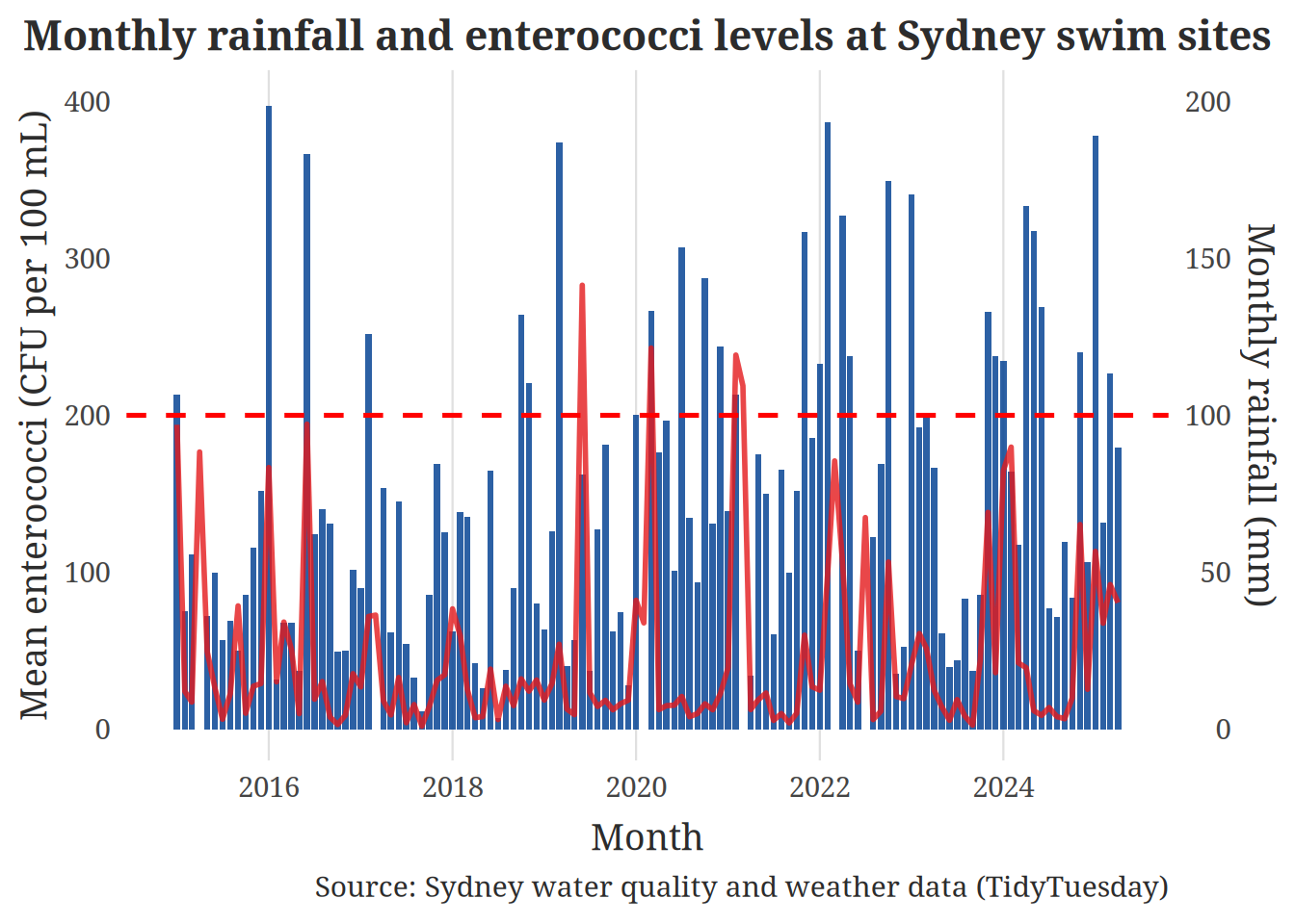
#Figure 2

#Standardizing date columns
water_quality_df <- water_quality_df |>
  mutate(
    date = as_date(date),
    enterococci_cfu_100ml = as.numeric(enterococci_cfu_100ml)
  )

weather_df <- weather_df |>
  mutate(
    date = as_date(date),
    precipitation_mm = as.numeric(precipitation_mm)
  )

#Joining the two dfs
ww_joined <- water_quality_df |>
  left_join(
    weather_df %>% select(date, precipitation_mm),
    by = "date"
  )

df_boxplot <- ww_joined |>
  mutate(
    rain_cat = case_when(
      precipitation_mm == 0 ~ "No rain",
      precipitation_mm > 0 & precipitation_mm < 5 ~ "Light (0-5mm)",
      precipitation_mm >= 5 & precipitation_mm < 20 ~ "Moderate (5-20mm)",
      precipitation_mm >= 20 ~ "Heavy (20mm+)"
    )
  )
#Getting the top swim sites in case too many to facet by
top_sites <- df_boxplot |>
  count(swim_site, sort = TRUE) |>
  slice_head(n = 9) |>
  pull(swim_site)

unsafe_threshold <- 200

safety_label <- data.frame(
  swim_site = c("Boat Harbour", "Elouera Beach", "Queenscliff Beach"),
  rain_cat = factor(
    "No rain",
    levels = c("No rain", "Light (0-5mm)", "Moderate (5-20mm)", "Heavy (20mm+)")
  ),
  y = unsafe_threshold * 2,
  label = "Safety threshold"
)


df_boxplot |>
  filter(
    !is.na(rain_cat),
    !is.na(enterococci_cfu_100ml),
    enterococci_cfu_100ml > 0,
    swim_site %in% top_sites
  ) |>
  mutate(
    rain_cat = factor(
      rain_cat,
      levels = c(
        "No rain",
        "Light (0-5mm)",
        "Moderate (5-20mm)",
        "Heavy (20mm+)"
      )
    )
  ) |>
  ggplot(aes(
    x = rain_cat,
    y = enterococci_cfu_100ml
  )) +
  geom_boxplot(
    outlier.alpha = 0.2,
    outlier.size = 0.8,
    fill = "#f0f4f8",
    color = "#000000",
    linewidth = 0.4
  ) +
  geom_hline(
    yintercept = unsafe_threshold,
    linetype = "dashed",
    color = "red",
    linewidth = 0.6
  ) +
  scale_y_log10(
    labels = label_comma(),
    breaks = c(1, 10, 100, 1000, 10000, 100000)
  ) +
  scale_x_discrete(
    labels = c(
      "No rain" = "No rain",
      "Light (0-5mm)" = "Light\n(0-5mm)",
      "Moderate (5-20mm)" = "Moderate\n(5-20mm)",
      "Heavy (20mm+)" = "Heavy\n(20mm+)"
    ),
    expand = expansion(add = c(1.2, 0.5))
  ) +
  geom_text(
    data = safety_label,
    aes(x = -Inf, y = y, label = label),
    hjust = -0.1,
    size = 2.5,
    fontface = "italic",
    family = "Georgia",
    inherit.aes = FALSE
  ) +
  facet_wrap(~swim_site, ncol = 3) +
  labs(
    title = "Distribution of Enterococci Levels at Various Swim Sites by Rainfall Category",
    x = "Daily rainfall category",
    y = "Enterococci level (CFU per 100 mL, log scale)",
    caption = "CFU = Colony Forming Units, measure of bacterial concentration.\nSource: Sydney water quality and weather data (TidyTuesday)"
  ) +
  theme_beach()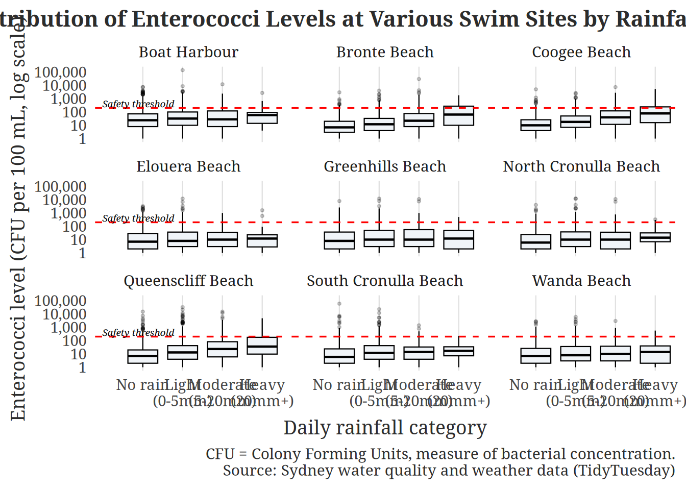
Discussion
Based on our graphs, it is evident that enterococci levels across all nine Sydney beaches show a clear and consistent pattern: bacterial concentrations rise notably with increasing rainfall. Under drier conditions, median levels at most sites sit well below the safety threshold of 200 CFU per 100 mL, suggesting that on rain‑free days the majority of these beaches are generally safe for swimming. However, as rainfall intensifies, particularly in the “Moderate (5–20 mm)” and “Heavy (20 mm+)” categories, median levels rise and the upper whiskers of the distributions frequently land above the red dashed safety threshold, indicating a substantially elevated risk of unsafe water conditions.
In the boxplot, Boat Harbour stands out as an outlier, with baseline enterococci levels already near or above the threshold even on dry days, pointing to persistent contamination sources independent of rainfall. Sites like Elouera, Greenhills, and North Cronulla Beach reamin comparatively cleaner across all rainfall categories, with medians staying below 100 CFU per 100 mL even after heavy rain, although extreme outliers above 10,000 CFU are visible across almost every beach and rainfall condition, highlighting that occasional severe contamination events can occur unpredictably.
Question 2 Does the effect of rainfall on enterococci concentration differ across regions?
Introduction
Rainfall can influence water quality because it washes pollutants, bacteria, and other contaminants from urban areas into nearby waterways. When rainfall enters water systems, it often can carry bacteria into beaches and swimming areas, increasing the concentration of microorganisms such as enterococci. Enterococci levels are commonly used as an indicator of microbial contamination which cna be potential health risks for swimmers. In this analysis, we will investigate if the relationship between rainfall and water quality differs across regions of Sydney. Specifically, we examine whether some regions experience larger increases in unsafe water conditions following heavy rainfall compared to dry days.
To answer this question, we will be using two datasets, a water quality dataset containing enterococci measurements at Sydney swim sites and a weather dataset containing daily precipitation levels. After cleaning and joining these datasets by date, we will identify days with heavy rainfall and compare the proportion of unsafe water samples across different regions. This question is important because regional differences in contamination risk could help people identify areas that are more vulnerable to rainfall driven pollution and can inform public health decisions about swimming safety.
Approach
Visualization 1:
To investigate how rainfall influences enterococci contamination and whether certain regions face greater risk, we need to identify each date as being “After Rain” day or “Dry” day. Enterococci bacteria are commonly washed into waterways through surface runoff during rain events; however because there if often a time lag between when it rains and when contamination level peaks (24-48 hours after a raining event), we decided to define “After Rain” as being any day where there is measurable rain (more than 1mm) as well as the two days that follow. Conversely, a “Dry” day is one that falls at least three full days after the most recent rain event, giving conditions enough time to return to a baseline state.
For the visualization itself, we chose a ridgeline plot to compare enterococci distributions across “After Rain” and “Dry” conditions, faceted by region. Given the large number of dates in the dataset, a time series would be far too cluttered to reveal meaningful patterns. Ridgeline plots instead show the full shape of the distribution — including its spread, skewness, and central tendency — making it easy to see at a glance whether a region’s contamination levels shift substantially after rainfall.
Visualization 2:
We decided to create a bar chart to compare the percentage of unsafe samples on dry days versus heavy rainfall days across regions. This plot’s purpose is to highlight whether some regions experience a higher contamination risk after heavy rainfall. This answers our question “Does the effect of rainfall on enterococci concentration differ across regions?” by showcases not only how the effects on different regions differ but also informing the viewer on which regions are considered “unsafe” or “safe” through a simple side by side comparison. A bar chart is appropriate since it makes it easy to see the percetages of unsafe water conditions while clearing identifying the different categories. The color mapping allows viewers to quickly identify differences in risk between dry and rainy conditions.
Analysis
# Classify rain days and non-rain days
weather_windowed <- weather_df |>
  mutate(date = as.Date(date)) |>
  arrange(latitude, longitude, date) |>
  group_by(latitude, longitude) |>
  mutate(
    max_rain_3d = rollapplyr(precipitation_mm, width = 3, FUN = max, fill = 0),

    # Define 'After Rain' if ANY of those 3 days had > 1mm of rain
    rain_event = ifelse(max_rain_3d > 1, "After Rain", "Dry")
  ) |>
  ungroup()

# Spatial Mapping: Spatially mapping the coordinates in the two datasets. Since there might be decrepancies between coordinate, we are mapping to coordinate that closest match one another
sites_sf <- water_quality_df |>
  distinct(swim_site, latitude, longitude) |>
  st_as_sf(coords = c("longitude", "latitude"), crs = 4326)

weather_locs_sf <- weather_windowed |>
  distinct(latitude, longitude) |>
  st_as_sf(coords = c("longitude", "latitude"), crs = 4326)

nearest_idx <- st_nearest_feature(sites_sf, weather_locs_sf)

site_map <- sites_sf |>
  st_drop_geometry() |>
  mutate(
    w_lat = st_coordinates(weather_locs_sf)[nearest_idx, 2],
    w_long = st_coordinates(weather_locs_sf)[nearest_idx, 1]
  )

#Joining the two datasets by date and (longitude, latitude)
final_data_3day <- water_quality_df |>
  mutate(date = as.Date(date)) |>
  left_join(site_map, by = "swim_site") |>
  left_join(
    weather_windowed,
    by = c("date" = "date", "w_lat" = "latitude", "w_long" = "longitude")
  )

# 1. Prepare data
ridge_data <- final_data_3day |>
  filter(
    !is.na(rain_event),
    !is.na(enterococci_cfu_100ml),
    enterococci_cfu_100ml >= 0
  ) |>
  mutate(region = reorder(region, enterococci_cfu_100ml, FUN = median))

# 2. Create Ridgeline Plot
ggplot(
  ridge_data,
  aes(x = enterococci_cfu_100ml, y = region, fill = rain_event)
) +
  # stat_density_ridges creates the 'mountain' shapes
  stat_density_ridges(
    aes(scale = 0.9),
    alpha = 0.7,
    quantile_lines = TRUE,
    quantiles = 2,
    color = "white"
  ) +

  # Logging enterococci level as raw number is too big
  scale_x_continuous(
    trans = "pseudo_log",
    breaks = c(0, 10, 100, 1000, 10000),
    labels = label_comma(),
    expand = c(0, 0)
  ) +

  scale_fill_manual(values = c("After Rain" = "#b31b1b", "Dry" = "#d3d3d3")) +

  # Add the 'Danger Zone' threshold line
  geom_vline(
    xintercept = 200,
    linetype = "dashed",
    color = "black",
    alpha = 0.6
  ) +

  labs(
    title = "Regional Enterococci Density: Dry vs. After Rain",
    subtitle = "Dry: <1mm rain over 72h | After Rain: >1mm precipitation within a 3-day rolling window",
    x = "Enterococci (CFU/100ml)",
    y = NULL,
    fill = "Condition"
  ) +
  theme_beach()
Picking joint bandwidth of 0.251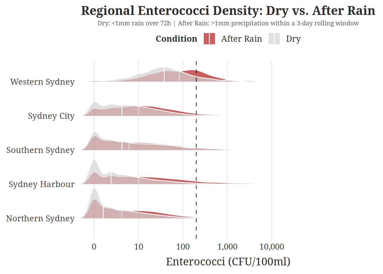
#visualization 2

#thresholds for safe water (cited in references)
unsafe_cfu <- 200
#heavy rainfall threshold decided by team
heavy_rain_mm <- 20

#cleaning datasets
water_clean <- water_quality_df |>
  mutate(
    date = as.Date(date),
    enterococci_cfu_100ml = as.numeric(enterococci_cfu_100ml)
  )

weather_clean <- weather_df |>
  mutate(
    date = as.Date(date),
    precipitation_mm = as.numeric(precipitation_mm)
  ) |>
  select(date, precipitation_mm) |>
  distinct()

#joining datasets
ww_joined <- water_clean |>
  left_join(weather_clean, by = "date") |>
  mutate(
    unsafe = enterococci_cfu_100ml > unsafe_cfu,
    rain_condition = case_when(
      precipitation_mm == 0 ~ "Dry",
      precipitation_mm >= heavy_rain_mm ~ "Heavy rain",
      TRUE ~ NA_character_
    ),
    rain_condition = factor(rain_condition, levels = c("Dry", "Heavy rain"))
  )

#summarizing data
risk_by_region <- ww_joined |>
  filter(
    !is.na(region),
    !is.na(rain_condition),
    !is.na(unsafe)
  ) |>
  group_by(region, rain_condition) |>
  summarize(
    pct_unsafe = mean(unsafe),
    n_samples = n()
  )
`summarise()` has regrouped the output.
ℹ Summaries were computed grouped by region and rain_condition.
ℹ Output is grouped by region.
ℹ Use `summarise(.groups = "drop_last")` to silence this message.
ℹ Use `summarise(.by = c(region, rain_condition))` for per-operation grouping
(`?dplyr::dplyr_by`) instead.#plotting side by side bar graph
risk_by_region |>
ggplot(aes(x = region, y = pct_unsafe, fill = rain_condition)) +
geom_col(position = "dodge") +
scale_y_continuous(labels = percent_format()) +
labs(
title = "Unsafe water quality risk on dry vs heavy rain days",
subtitle = "Unsafe if enterococci > 200 CFU/100 mL, heavy rain ≥ 20 mm",
x = NULL,
y = "Percent unsafe",
fill = NULL
) +
theme_beach() +
theme(axis.text.x = element_text(angle = 30, hjust = 1))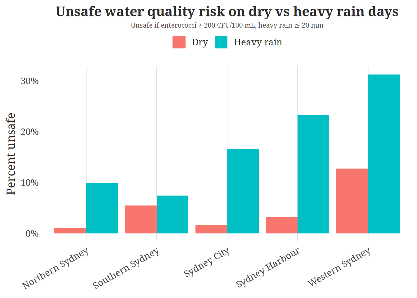
Discussion (Q2)
This ridgeline plot shows a clear and consistent link between recent rainfall and a spike in Enterococci levels across all five Sydney regions. By tracking bacterial density over a 3-day window, we can see that rain pushes the bacterial concentration distribution to the right for all regions. Western Sydney stands out as the most severely impacted area in this analysis. Unlike other regions that simply show increased variance, Western Sydney experiences a wholesale shift in its median concentration. So while all regions are susceptible to an increase in Enterococci levels after a rain event, the impact on Western Sydney is particularly severe.
visualization 2 shows that when it rains there is consistenly higher percentages of unsafe water quality compared to dry days. This pattern is especially apparent in regions such as Western Sydney and Sydney Harbour where the percentage of unsafe samples rises substaintially after heavy rain. A possible reason why there is a higher percentage of unsafe water after rainfal is that heavy rain can carry storm water runoff that carries pollutants, waste, and bacteria into water systems. Areas with more urban development that discharge directly into swomming areas may experience a larger spike in contamination. This may explain why some regions experience greater increase in unsafe water levels than others.
Presentation
Our presentation can be found here.
Data
Both datasets below were retrieved from one dataframe of TidyTuesday project.
TidyTuesday. 2025. Sydney Beach Water Quality Data. Enterococci measurements collected from Sydney swimming sites. Retrieved March 2026 from:https://github.com/rfordatascience/tidytuesday/blob/main/data/2025/2025-05-20/readme.md
TidyTuesday. 2025. Sydney Weather Data. Daily precipitation measurements used to examine rainfall patterns. Retrieved March 2026 from: https://github.com/rfordatascience/tidytuesday/blob/main/data/2025/2025-05-20/readme.md
References
List any references here. You should, at a minimum, list your data source.
TidyTuesday 2025 Sydney Beach Water Quality Data Retrieved March 2026 from: https://github.com/rfordatascience/tidytuesday/blob/main/data/2025/2025-05-20/readme.md
TidyTuesday 2025 Sydney Weather Data Retrieved March 2026 from: https://github.com/rfordatascience/tidytuesday/blob/main/data/2025/2025-05-20/readme.md
Water samples are classified as unsafe when enterococci concentrations exceed 200 CFU per 100 mL, consistent with Australian recreational water quality guidelines. Source: National Health and Medical Research Council. 2008. Guidelines for Managing Risks in Recreational Water. Australian Government. https://www.ccaquapark.com.au/water-quality