library(tidyverse)
library(skimr)
library(lubridate)
library(scales)project-elegant-buneary
Exploration
Objective(s)
State the question(s) you are answering or the problem(s) you are solving clearly.
Data collection and cleaning
Have an initial draft of your data cleaning appendix. Document every step that takes your raw data file(s) and turns it into the analysis-ready data set that you would submit with your final project. Include text narrative describing your data collection (downloading, scraping, surveys, etc) and any additional data curation/cleaning (merging data frames, filtering, transformations of variables, etc). Include code for data curation/cleaning, but not collection.
# load data and skim
airlines <- read_csv("data/airlines.csv")
Rows: 4408 Columns: 24
── Column specification ────────────────────────────────────────────────────────
Delimiter: ","
chr (5): Airport.Code, Airport.Name, Time.Label, Time.Month Name, Statistic...
dbl (19): Time.Month, Time.Year, Statistics.# of Delays.Carrier, Statistics....
ℹ Use `spec()` to retrieve the full column specification for this data.
ℹ Specify the column types or set `show_col_types = FALSE` to quiet this message.skimr::skim(airlines)| Name | airlines |
| Number of rows | 4408 |
| Number of columns | 24 |
| _______________________ | |
| Column type frequency: | |
| character | 5 |
| numeric | 19 |
| ________________________ | |
| Group variables | None |
Variable type: character
| skim_variable | n_missing | complete_rate | min | max | empty | n_unique | whitespace |
|---|---|---|---|---|---|---|---|
| Airport.Code | 0 | 1 | 3 | 3 | 0 | 29 | 0 |
| Airport.Name | 0 | 1 | 23 | 67 | 0 | 29 | 0 |
| Time.Label | 0 | 1 | 7 | 7 | 0 | 152 | 0 |
| Time.Month Name | 0 | 1 | 3 | 9 | 0 | 12 | 0 |
| Statistics.Carriers.Names | 0 | 1 | 68 | 412 | 0 | 841 | 0 |
Variable type: numeric
| skim_variable | n_missing | complete_rate | mean | sd | p0 | p25 | p50 | p75 | p100 | hist |
|---|---|---|---|---|---|---|---|---|---|---|
| Time.Month | 0 | 1 | 6.58 | 3.46 | 1 | 4.00 | 7.0 | 10.00 | 12 | ▇▅▅▅▇ |
| Time.Year | 0 | 1 | 2009.24 | 3.67 | 2003 | 2006.00 | 2009.0 | 2012.00 | 2016 | ▇▇▅▇▆ |
| Statistics.# of Delays.Carrier | 0 | 1 | 574.63 | 329.62 | 112 | 358.00 | 476.0 | 692.00 | 3087 | ▇▂▁▁▁ |
| Statistics.# of Delays.Late Aircraft | 0 | 1 | 789.08 | 561.80 | 86 | 425.00 | 618.5 | 959.00 | 4483 | ▇▂▁▁▁ |
| Statistics.# of Delays.National Aviation System | 0 | 1 | 954.58 | 921.91 | 61 | 399.00 | 667.5 | 1166.00 | 9066 | ▇▁▁▁▁ |
| Statistics.# of Delays.Security | 0 | 1 | 5.58 | 6.01 | -1 | 2.00 | 4.0 | 7.00 | 94 | ▇▁▁▁▁ |
| Statistics.# of Delays.Weather | 0 | 1 | 78.22 | 75.18 | 1 | 33.00 | 58.0 | 98.00 | 812 | ▇▁▁▁▁ |
| Statistics.Carriers.Total | 0 | 1 | 12.25 | 2.29 | 3 | 11.00 | 12.0 | 14.00 | 18 | ▁▂▇▇▁ |
| Statistics.Flights.Cancelled | 0 | 1 | 213.56 | 288.87 | 3 | 58.00 | 123.0 | 250.00 | 3680 | ▇▁▁▁▁ |
| Statistics.Flights.Delayed | 0 | 1 | 2402.00 | 1710.95 | 283 | 1298.75 | 1899.0 | 2950.00 | 13699 | ▇▂▁▁▁ |
| Statistics.Flights.Diverted | 0 | 1 | 27.88 | 36.36 | 0 | 8.00 | 15.0 | 32.00 | 442 | ▇▁▁▁▁ |
| Statistics.Flights.On Time | 0 | 1 | 9254.42 | 5337.21 | 2003 | 5708.75 | 7477.0 | 10991.50 | 31468 | ▇▅▂▁▁ |
| Statistics.Flights.Total | 0 | 1 | 11897.86 | 6861.69 | 2533 | 7400.00 | 9739.5 | 13842.50 | 38241 | ▇▆▂▁▁ |
| Statistics.Minutes Delayed.Carrier | 0 | 1 | 35021.37 | 24327.72 | 6016 | 19530.75 | 27782.0 | 41606.00 | 220796 | ▇▂▁▁▁ |
| Statistics.Minutes Delayed.Late Aircraft | 0 | 1 | 49410.27 | 38750.02 | 5121 | 25084.25 | 37483.0 | 59951.25 | 345456 | ▇▁▁▁▁ |
| Statistics.Minutes Delayed.National Aviation System | 0 | 1 | 45077.11 | 57636.75 | 2183 | 14389.00 | 25762.0 | 50362.00 | 602479 | ▇▁▁▁▁ |
| Statistics.Minutes Delayed.Security | 0 | 1 | 211.77 | 257.17 | 0 | 65.00 | 141.0 | 274.00 | 4949 | ▇▁▁▁▁ |
| Statistics.Minutes Delayed.Total | 0 | 1 | 135997.54 | 113972.28 | 14752 | 65444.75 | 100711.0 | 164294.75 | 989367 | ▇▁▁▁▁ |
| Statistics.Minutes Delayed.Weather | 0 | 1 | 6276.98 | 6477.42 | 46 | 2310.75 | 4298.5 | 7846.00 | 76770 | ▇▁▁▁▁ |
# fix column names by using saplly()
snake_case <- function(x) {
  x <- gsub(" ", "_", x)
  x <- gsub("#", "_", x)
  x <- gsub("\\.", "_", x)
  x <- gsub("___", "_", x)
  x <- gsub("__", "_", x)
  x <- tolower(x)
  return(x)
}

colnames(airlines) <- sapply(colnames(airlines), snake_case)

# remove "statistics_" from column names
colnames(airlines) <- gsub("statistics_of_", "", colnames(airlines))
colnames(airlines) <- gsub("statistics_", "", colnames(airlines))
airlines_clean <- airlines |>
separate_rows(carriers_names, sep = ",") |>
rename(airline = carriers_names) |>
separate(
col = airport_name,
into = c("state", "country", "airport_name"),
sep = "[,:]"
) |>
rename(
month_num = time_month,
month_name = time_month_name,
year = time_year
)
delay_reason <- airlines |>
select(starts_with("delays_"))
airlien_clean <- airlines_clean |>
mutate(
month_num = as.numeric(month_num),
year = as.numeric(year)
)# save cleaned data
write_csv(airlines_clean, "data/airlines_cleaned.csv")Data description
The dataset used for the analysis of flight data in the United States is a comprehensive collection of statistics related to flights, delays, carriers, and airports. This analysis-ready dataset was originally collected from the U.S. Department of Transportation’s Bureau of Transportation Statistics (BTS) and is part of the CORGIS (Collection of Really Great, Interesting, and Situated Datasets) project. The dataset provides valuable insights into the aviation industry and its impact on passengers’ travel experiences.
The dataset used for the analysis of flight data in the United States has undergone a series of cleaning and preprocessing steps to ensure it is analysis-ready. We did cleaning by standardizing column names to snake_case and reshaping the data for easier analysis, and we also reshaped the data by using the pivot_longer() function to make it easier to analyze. For the airport name, we are separating from one columns to three, for example, for “Atlanta, GA: Hartsfield-Jackson Atlanta International” the result will be “Atlanta”, “GA”, and “Hartsfield-Jackson Atlanta International”. There were no NA values in the dataset, so we did not need to remove any rows or columns. The dataset is now ready for analysis.
Data limitations
Identify any potential problems with your dataset.
- The dataset could be inaccurate. The accuracy of the data is paramount to the success of the project. Any inaccuracies in the dataset, such as incorrect flight statistics or airport information, could lead to incorrect conclusions.
- There will also be temporal limitations. The dataset only covers data from June 2003 to Jan 2016, and this temporal limitation may affect the generalizability of findings, especially when analyzing contemporary trends.
Exploratory data analysis
Perform an (initial) exploratory data analysis.
library(ggplot2)
airlines_clean <- read_csv("data/airlines_cleaned.csv")
Rows: 54013 Columns: 26
── Column specification ────────────────────────────────────────────────────────
Delimiter: ","
chr (7): airport_code, state, country, airport_name, time_label, month_name...
dbl (19): month_num, year, delays_carrier, delays_late_aircraft, delays_nati...
ℹ Use `spec()` to retrieve the full column specification for this data.
ℹ Specify the column types or set `show_col_types = FALSE` to quiet this message.glimpse(airlines_clean)Rows: 54,013
Columns: 26
$ airport_code <chr> "ATL", "ATL", "ATL", "ATL", "…
$ state <chr> "Atlanta", "Atlanta", "Atlant…
$ country <chr> "GA", "GA", "GA", "GA", "GA",…
$ airport_name <chr> "Hartsfield-Jackson Atlanta I…
$ time_label <chr> "2003/06", "2003/06", "2003/0…
$ month_num <dbl> 6, 6, 6, 6, 6, 6, 6, 6, 6, 6,…
$ month_name <chr> "June", "June", "June", "June…
$ year <dbl> 2003, 2003, 2003, 2003, 2003,…
$ delays_carrier <dbl> 1009, 1009, 1009, 1009, 1009,…
$ delays_late_aircraft <dbl> 1275, 1275, 1275, 1275, 1275,…
$ delays_national_aviation_system <dbl> 3217, 3217, 3217, 3217, 3217,…
$ delays_security <dbl> 17, 17, 17, 17, 17, 17, 17, 1…
$ delays_weather <dbl> 328, 328, 328, 328, 328, 328,…
$ airline <chr> "American Airlines Inc.", "Je…
$ carriers_total <dbl> 11, 11, 11, 11, 11, 11, 11, 1…
$ flights_cancelled <dbl> 216, 216, 216, 216, 216, 216,…
$ flights_delayed <dbl> 5843, 5843, 5843, 5843, 5843,…
$ flights_diverted <dbl> 27, 27, 27, 27, 27, 27, 27, 2…
$ flights_on_time <dbl> 23974, 23974, 23974, 23974, 2…
$ flights_total <dbl> 30060, 30060, 30060, 30060, 3…
$ minutes_delayed_carrier <dbl> 61606, 61606, 61606, 61606, 6…
$ minutes_delayed_late_aircraft <dbl> 68335, 68335, 68335, 68335, 6…
$ minutes_delayed_national_aviation_system <dbl> 118831, 118831, 118831, 11883…
$ minutes_delayed_security <dbl> 518, 518, 518, 518, 518, 518,…
$ minutes_delayed_total <dbl> 268764, 268764, 268764, 26876…
$ minutes_delayed_weather <dbl> 19474, 19474, 19474, 19474, 1…carrier_summary <- airlines_clean |>
group_by(airline) |>
summarize(total_hours_delayed = sum(minutes_delayed_total) / 60, .groups = "drop") |>
ungroup()
# Create a bar chart with carriers sorted from smallest to largest total hours delayed
ggplot(carrier_summary, aes(x = reorder(airline, total_hours_delayed), y = total_hours_delayed)) +
geom_bar(stat = "identity", color = "#6F8FAF", fill = "#A7C7E7") +
labs(
title = "Total Hours Delayed by Carrier (Smallest to Largest)",
x = "Carrier",
y = "Total Hours Delayed"
) +
theme_minimal() +
coord_flip() +
scale_y_continuous(labels = scales::comma)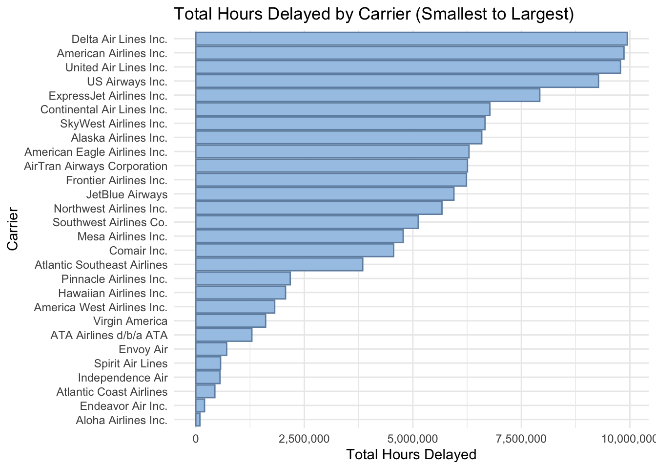
airlines_clean |>
  filter(airline == "American Airlines Inc.") |>
  group_by(year) |>
  summarise(percentage_delayed = (sum(flights_delayed) / sum(flights_on_time))) |>
  drop_na() |>
  ggplot(mapping = aes(x = year, y = percentage_delayed)) +
  geom_line(aes(color = "pink")) +
  geom_point(aes(color = "turquoise"), size = 2.5) +
  labs(
    x = "Year",
    y = "Percentage of Flights Delayed",
    title = "Percentage of Flights Delayed for American Airlines Over the Years"
  ) +
  theme_minimal() +
  theme(legend.position = "none") +
  scale_y_continuous(labels = scales::percent)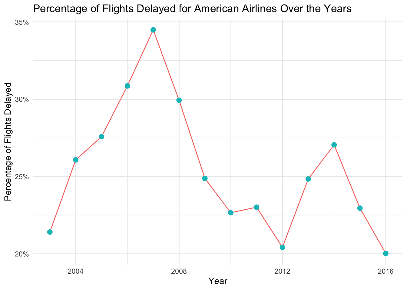
filtered_df <- airlines_clean |>
  filter(year >= 2010 & year <= 2015) |>
  group_by(airline) |>
  summarise(
    average_delay = mean(delays_late_aircraft) / mean(flights_total)
  ) |>
  drop_na() |>
  print()
# A tibble: 22 × 2
airline average_delay
<chr> <dbl>
1 AirTran Airways Corporation 0.0660
2 Alaska Airlines Inc. 0.0685
3 American Airlines Inc. 0.0670
4 American Eagle Airlines Inc. 0.0658
5 Atlantic Southeast Airlines 0.0620
6 Comair Inc. 0.0611
7 Continental Air Lines Inc. 0.0638
8 Delta Air Lines Inc. 0.0673
9 Endeavor Air Inc. 0.0675
10 Envoy Air 0.0693
# ℹ 12 more rowsairline_plot_3 <- ggplot(
data = filtered_df,
aes(x = reorder(airline, average_delay), y = average_delay)
) +
geom_bar(stat = "identity", fill = "#A7C7E7", color = "#6F8FAF") +
labs(
x = "Airline",
y = "Average Percentage of Flights Delayed",
title = "Average Percentage of Flights Delayed per Airline"
) +
theme_minimal() +
theme(axis.text.x = element_text(angle = 90, vjust = 0.5, hjust = 1)) +
scale_y_continuous(labels = scales::percent_format(accuracy = 1))
airline_plot_3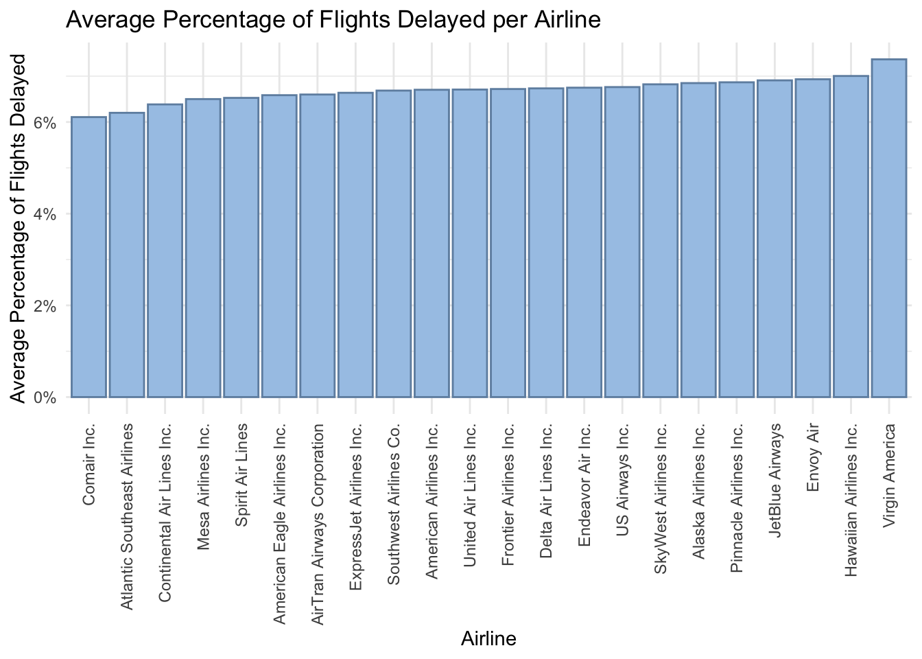
Questions for reviewers
List specific questions for your peer reviewers and project mentor to answer in giving you feedback on this phase.
- Is the cleaned dataset analysis-ready?
- Are the visualizations clear and easy to understand?
- Are there any other visualizations that would be helpful to include? (e.g., a map of the United States showing the number of flights delayed by state, or a drop-down menu to select a specific carrier and see the percentage of flights delayed over time) We will use shiny app for the project by the way.