Unveiling Workforce Dynamics: Exploring Pay Disparities in Los Angeles 2022
Exploration
Objective(s)
We want to present an analysis of the workforce in the city of Los Angeles. Through an interactive web application we will delve into the diversity of the workforce and try to determine if there are disparities in payroll distribution based on different factors such as department, gender, and ethnicity for the year 2022.
# Calculate the average total pay for each categoryavg_department <- payroll_2022 |>group_by(DEPARTMENT_TITLE) |>summarize(avg_total_pay =mean(TOTAL_PAY))avg_gender <- payroll_2022 |>group_by(GENDER) |>summarize(avg_total_pay =mean(TOTAL_PAY))avg_ethnicity <- payroll_2022 |>group_by(ETHNICITY) |>summarize(avg_total_pay =mean(TOTAL_PAY))
We did the filter online. Since we are only looking at active full time jobs in 2022, we’ve filtered PAY_YEAR = 2022, EMPLOYMENT_TYPE = “FULL_TIME”, and JOB_STATUS = “ACTIVE” on the website. Because the dataset is too large to be uploaded on GitHub, we separated the dataset by each department number (into 10 different datasets) and uploaded them on GitHub. We then combine them into one dataset using a map function because all the dataset files are named similarly except their department numbers. All columns are already in snake_case and their appropriate data types. The dataset is then turned it into the analysis-ready dataset: avg_department, avg_gender, and avg_ethnicity as we calculated the average total pay for each category (total pay by department, gender, and ethnicity).
Data description
We have taken the data filtering out only full-time, active workers for each department logged in the dataset prior to cleaning. After attaining a dataset for each department we joined each dataset together so that we can have a centralized location for all of our data, easing the process of further analysis.
Data limitations
There are two limitations for this dataset on this phase. The first one is if the position is unionized or not, and the second one is the work time and overtime frequency. For the first one, unionized position will have different pay structures, benefits, and work rules compared to non-unionized employees. Without this information, it becomes challenging to perform comprehensive labor cost analysis and budgeting. Work time and overtime frequency will also affect the payroll. In general, the more hours worked, especially overtime hours, the higher the employee’s earnings will be.
Exploratory data analysis
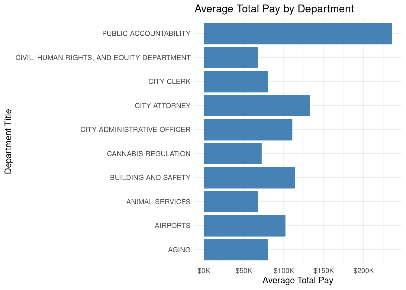
ggplot(avg_department, aes(x = avg_total_pay, y = DEPARTMENT_TITLE)) +geom_col(fill ="steelblue") +scale_x_continuous(labels = scales::dollar_format(scale =1e-3, suffix ="K")) +labs(x ="Average Total Pay",y ="Department Title",title ="Average Total Pay by Department" ) +theme_minimal()
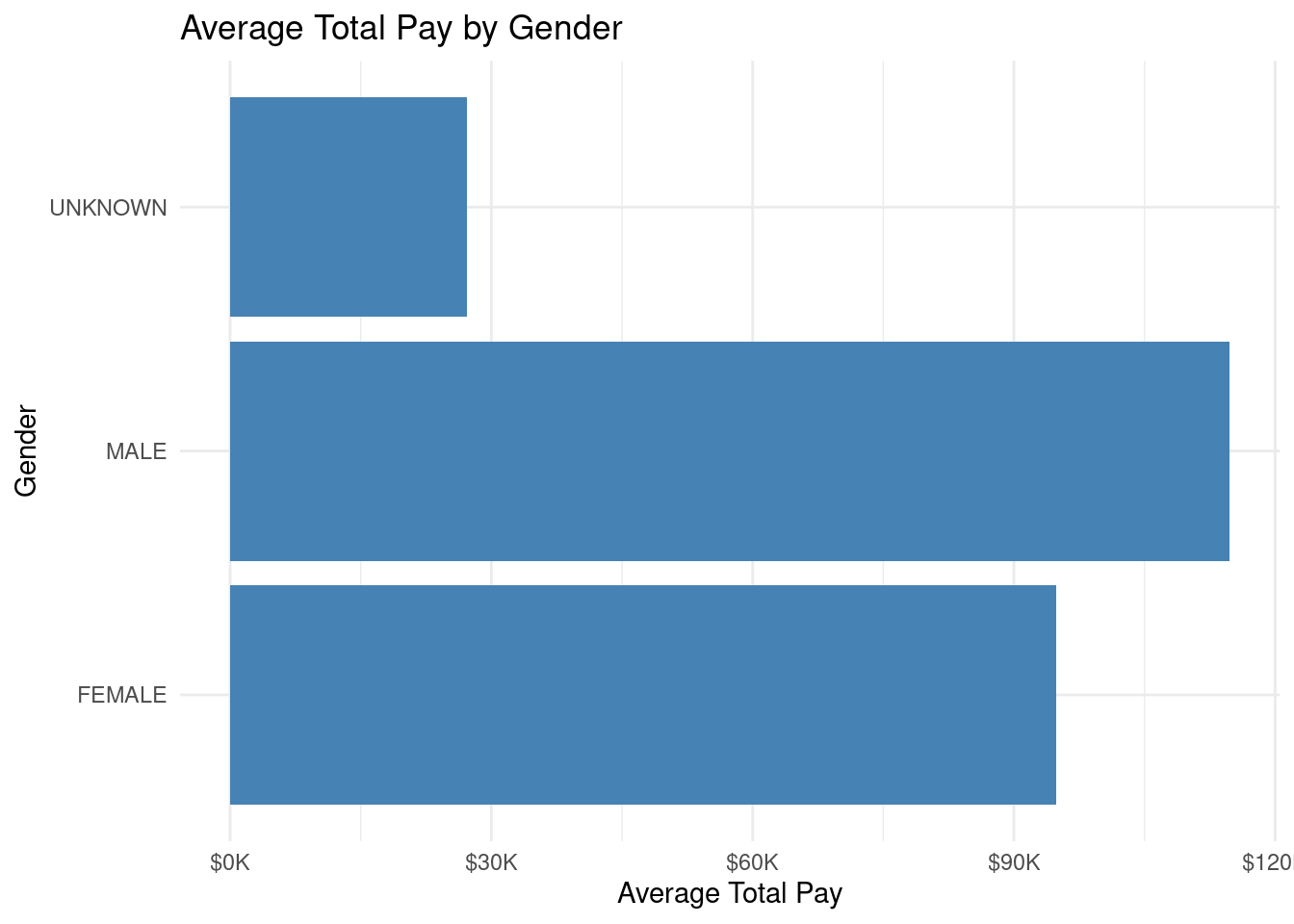
ggplot(avg_gender, aes(x = avg_total_pay, y = GENDER)) +geom_col(fill ="steelblue") +scale_x_continuous(labels = scales::dollar_format(scale =1e-3, suffix ="K")) +labs(x ="Average Total Pay",y ="Gender",title ="Average Total Pay by Gender" ) +theme_minimal()
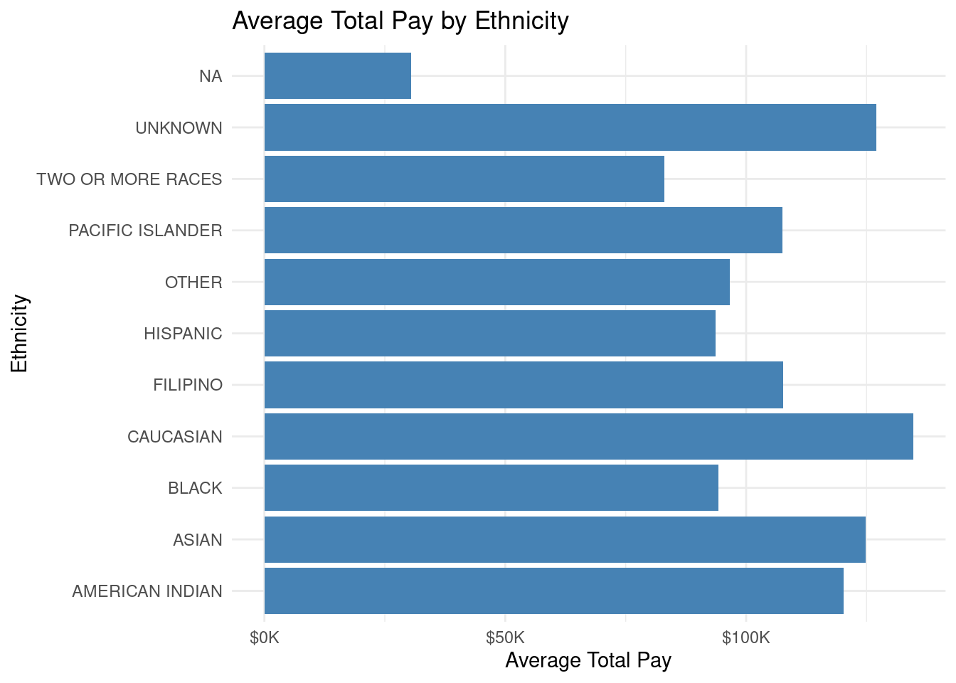
ggplot(avg_ethnicity, aes(x = avg_total_pay, y = ETHNICITY)) +geom_col(fill ="steelblue") +scale_x_continuous(labels = scales::dollar_format(scale =1e-3, suffix ="K")) +labs(x ="Average Total Pay",y ="Ethnicity",title ="Average Total Pay by Ethnicity" ) +theme_minimal()
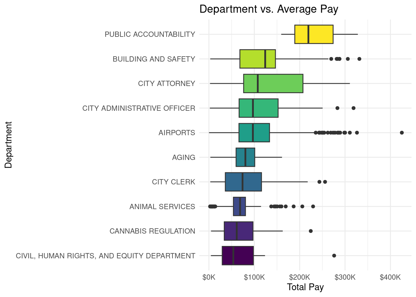
department_total_pay <- payroll_2022 |>select(DEPARTMENT_TITLE, TOTAL_PAY) |>mutate(DEPARTMENT_TITLE =reorder(DEPARTMENT_TITLE, TOTAL_PAY, FUN = median))ggplot(department_total_pay, aes(x = TOTAL_PAY, y = DEPARTMENT_TITLE, fill = DEPARTMENT_TITLE)) +geom_boxplot(show.legend =FALSE) +labs(title ="Department vs. Average Pay",x ="Total Pay",y ="Department") +scale_x_continuous(labels = scales::dollar_format(scale =1e-3, suffix ="K")) +scale_fill_viridis_d() +theme_minimal()
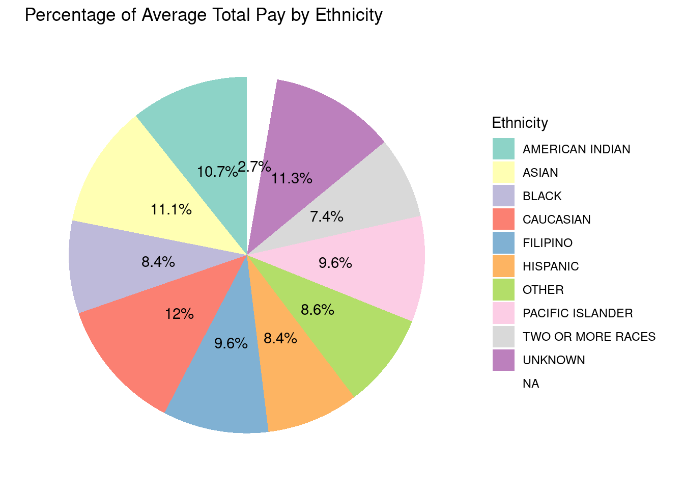
# Calculate the total average paytotal_avg_pay <-sum(avg_ethnicity$avg_total_pay)# Calculate the percentage for each ethnicityavg_ethnicity$percentage <- (avg_ethnicity$avg_total_pay / total_avg_pay) *100# Create the pie chartggplot(avg_ethnicity, aes(x ="", y = percentage, fill = ETHNICITY)) +geom_bar(stat ="identity", width =1) +coord_polar(theta ="y") +scale_fill_brewer(palette ="Set3") +# Optional: Adds a color palettelabs(x ="",y ="",title ="Percentage of Average Total Pay by Ethnicity",fill ="Ethnicity" ) +theme_minimal() +theme(axis.line =element_blank(),axis.text =element_blank(),axis.ticks =element_blank(),axis.title =element_blank(),panel.grid =element_blank()) +geom_text(aes(label =paste0(round(percentage, 1), "%")), position =position_stack(vjust =0.5))
Department Analysis: In our initial exploratory data analysis (EDA), we examined the distribution of average pay across various city departments in Los Angeles for the year 2022. We found that the average total pay across all departments hovers around $100,000. The department “Public Accountability” stands out with the highest average pay at $235,587, while the “Aging” department has the lowest average pay at $79,588.
Gender Analysis: Our EDA also involved an analysis of gender-based disparities in pay. On average, males earn significantly more with an average total pay of approximately $114,808, compared to females whose average is around $94,807. However, it’s important to note that there is a category labeled “Unknown” with a substantially lower average pay of $27,171, which warrants further investigation.
Ethnicity Analysis: In our exploration of workforce diversity, we analyzed average pay by ethnicity. “Caucasian” employees had the highest average pay at $134,676, while “NA” (Not Available) recorded the lowest average pay at $30,448. “Unknown” ethnicity had an average pay of $126,984, indicating a need for further clarification.
Visualizations, such as bar charts, box plots, and pie charts, can effectively display these differences and help identify any outliers within each department (using box plots). This initial analysis sets the stage for a deeper examination of potential disparities in pay across different departments.
Questions for reviewers
Based on our understanding, gender and ethnicity will not affect total pay, but job title and department will affect it. If we want to add the prediction of total pay for the next year, what model can we use based on data we have already collected?
Are there still some elements that will affect total pay?