Michelle D. Davies

In Lab 0, I set up my working environment for my robot, I verified that I have all of the needed components in my kit, and I built the base of my robot, which you will see in the Lab 1 section.

My Working Environment

For my work area, I have both desk space and easily accessible space on my tile floors to allow the robot to move while connected to its USB cable.

My Kit

In Lab 1, we began to program the Arduino to read, interpret data from a sensor, and actuate responses to the data collected. THis lab helps us gain practice in working with photoresistors in preparation of Lab 2.

Important Information/Attachments to Begin

• Lab 1 Handwritten Scrap Paper
• The maximum voltage, with respect to ground, that can be applied to any pin is VDD + 0.5V.
• Vref = Vin = 5V

Prototyping the Circuit with 1 Photoresistor

To begin, I built the simple version of a photoresistor circuit so that I could get used to working with the photoresistor on both a hardware and software level, and well as get some readings from my testing environment based on how I illuminate it. This photoresistor is attached to the analog pin A0.

Photoresistor Readings under normal conditions

Photosensor Data on Serial Monitor, Normal, Page 1

Photosensor Data on Serial Monitor, Normal, Page 2

Photosensor Data on Serial Monitor, Normal, Page 3

Photoresistor Readings with a central light sourse

Photosensor Data on Serial Monitor, Light Source, Page 1

Photosensor Data on Serial Monitor, Light Source, Page 2

Photosensor Data on Serial Monitor, Light Source, Page 3

Photosensor Data on Serial Monitor, Light Source, Page 4

Building the Real Circuit with both Photoresistors

Once I was comfortable with the circuit and the code needed to collect data from one of the photoresistors, I went ahead and modified the circuit to include both resistors.

After I added the second photoresistor to the circuit, I proceeded to write the code needed to read, distinguish and display the data from both sensors so that I can calibrate my readings for the semester. Analog pin A0 reads the data from the leftmost photoresistor, while analog pin A1 reads the data from the rightmost photoresistor. Writing this code required me to build upon the code for reading from one photoresistor, as well as introduce new concepts to have my code make and interpret measurements.

Among the most important concepts from this lab that with play a major role in future labs is the use of a Normalized Measurement of the relative light detected by the photoresistors. This is important because taking Normalized Measurements ("NM") ensures that we don't have to keep recalibrating the luminance for the area at each location the robot travels too.

Final Results, Summary & Takeaways, Next Steps

This is what my robot currently looks like:

Final Results for the Two Photoresistors Under Normal Testing Conditions (Out of 24 Trials)

Data Parameter	Photoresistor Data
Minimum Reading (L)	343 Lux
Minimum Reading (R)	811 Lux
Minimum Reading (NM, L)	0.30
Minimum Reading (NM, R)	0.70
Median Reading (L)	541 Lux
Median Reading (R)	898 Lux
Median NM Reading (L)	0.365
Median NM Reading (R)	0.635
Maximum Reading (L)	739 Lux
Maximum Reading (R)	985 Lux
Maximum Reading (NM, L)	0.43
Maximum Reading (NM, R)	0.57

Summary & Takeaways

In Lab 1, my biggest takeaway was that I gained a valuable foundation of how photoresistors work, as well better practices for collecting sensor data and setting up a smoother, better functioning ambient-responsive system by taking Normalized Measurements.

Next Steps

Now that I am getting NM readings that make sense and accurately respond to ambient stimulus, my next steps are to write out test cases for how my robots should move according to how I set the surrounding lighting. One way that I plan to maintain consistency in my test cases is by doing my labs at the same time in the same setting each week, i.e. Wednesdays at 7:30 in the same area of my room, and no changes in furniture arrangement or shadowing.

In Lab 2, we were tasked with using the results and progress we made in Lab 1 with the CdS photoresistors, combined with the motors and the h‐bridge to actuate the robot and turn it into a light‐following robot.

Important Information/Attachments to Begin

• Lab 2 ADC Measurement Results (mdd94.txt)

My Procedure for this Lab

1. I gathered results from interacting with the timing of the Analog to Digital Converter ("ADC") process Nano Every's ADC peripheral.
2. I wired and tested the connection of my H-Bridge.
3. I calibrated the motors for my robot's wheels.
4. I incorporated my work on the photosensor data from Lab 1 into this lab to actuate the appropriate response to my data (i.e. have the robot move according to the direction of a given light source).

"Playing with the ADC" Results

Data Parameter	Values from ADC
What is the default value of the ADC prescaler?	CLK_PER divided by 128
What is the prescaler that fixes the value of CLK_PER?	Division by 2
What is the default value of the PEN bit of the MCLKCTRLB register?	0 (Disabled), This means that no prescaler is used, so CLK_MAIN will be the clock signal directly from the 16/20 MHz clock.
What is the minimum allowable ADC prescaler that must be used for the CLK_PER signal corresponding to the 16 MHz signal of the oscillator, keeping in mind the allowed prescaler values in the CTRLC register?	CLK_PER divided by 16 - This is interesting because which this is the minimum guarenteed prescaler to work, we can see valid ADC outputs starting at CLK_PER divided by 8 (View data here).

Final Results, Summary & Takeaways, Next Steps

This is what my robot currently looks like:

Final Results / Test Cases:

As quoted and summarized from the Lab 2 Handout, here are the lab's main objectives:

• The robot's motion is to be smooth (i.e. no wiggling).
• "When the robot will be in normal lighting conditions, or when there is too much light everywhere, the robot will turn around in place, not knowing where to go. During this, the onboard LED on the Arduino will blink (ON for 500ms, OFF for 500ms, etc.)."
• "When bright (brighter) light hits the robot from one side or the other, the onboard LED will stop blinking, and the robot will move towards the bright light until the bright light is turned off again or the robot has turned sufficiently so that it faces the light, at which point the robot will move towards it in a straight line."
• "The above cycle is repeated depending on if the bright light is removed (i.e., returning the robot to normal lighting conditions), or if the bright light continues to shine (from straight ahead, or from either side of the robot), with the robot adapting as described above."

Picture 1: Circuit with H Bridge Wired

Video 1, From Part E: Wheels Turning in Free Motion (Serial Monitor Output Included)

Video 2, From Part G: Robot Moving Slowly in a Straight Line (Serial Monitor Output Included)

Video 3, From Part H: Robot Moving at Medium Speed in a Straight Line (Serial Monitor Output Included)

Video 4, From Part I: Robot Moving Given Lighting Conditions fron Photoresistors (Serial Monitor Output Included)

Summary & Takeaways

In Lab 2, my biggest takeaways were that (1) I need to back up my files/work more regularly, (2) the labs are getting more complicated and I need to continue to work towards weekly milestones along with my partner to finish, (3) I need to keep organizing my wiring for troubleshooting purposes, and finally, (4) writing helper functions with a lot of comments in my code is essential to my process for collecting and acting upon data.

Next Steps

Now that I have used the inputs that I configured in Lab 1 to actuate the directionality and motion of the robot's wheels for Lab 2, my next steps are to back up my work, store my circuit somewhere safe, and look into optimizing my circuit design and code more. One way that I plan to do this is by reviewing this lab weekly even as I move on to working on other phases of the semester labs.

In Lab 3, we were tasked with implementing and testing passive and active filters using the hardware that you have on hand, combined with your computer and MATLAB, and compare them to what is theoretically predicted. We also implemented and tested a bandpass filter that will be used on our robots in Lab 4.

My Procedure for this Lab

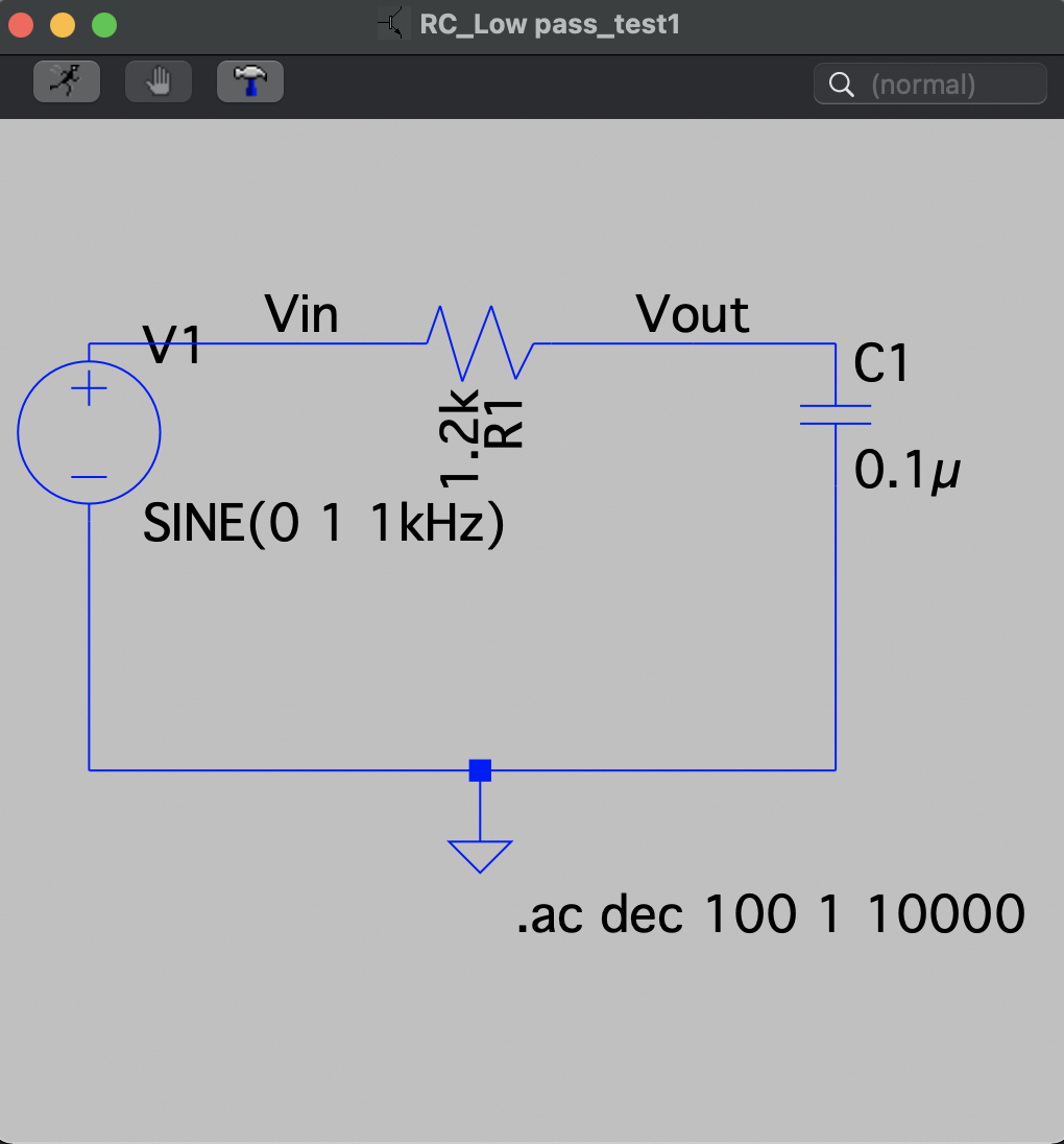
1. Sections 0-3 (04/06): Answer Questions on Canvas, Use LTSpice to Draw Low Pass and High Pass Filters, Build the Microphone Circuit, and Code the Arduino and MATLAB to Characterize Circuits
2. Sections 4-6 (04/13): Improve the Microphone Circuit, Test my Low Pass and High Pass Circuits, and Create a Bandpass Filter
3. Sections 7-9 (04/20): Setup FFT on Arduino, Complete Lab and submit deliverables.

Answering Questions on Canvas

Question	My Answer
Consider using TCA in a simple application of a periodic interrupt, as discussed in class. In this problem, you want to toggle the onboard LED every 135 ms (i.e., the LED is ON for 135 ms, then OFF for 135 ms, etc.). What is the number of clock ticks between the moment when the timer starts and the moment when the interrupt is triggered after 135 ms assuming that you use a TCA prescaler of 16 and your Nano's operating frequency is 16 MHz (no prescaler is used for the main clock)?	You cannot have this period of 135 ms with the given parameters.
Given that your Nano's operating frequency is 16 MHz (no prescaler is used for the main clock), what is (approximately) the longest possible achievable interrupt period for TCA?	4.096 millisecs
You have an application that involves using TCB (instance 0) in the Input Capture on Event mode. You want to use the Noise Cancellation feature of TCB, and you want the event edge detector to trigger the capture on falling edges. Which of the following (choose all that apply) can be used to set the appropriate register bits to set the three requirements above (Input Capture on Event mode, Noise Cancellation feature, trigger the capture on falling edges)?	TCB0.CTRLB |= TCB_CNTMODE_CAPT_gc; TCB0.EVCTRL |= TCB_CAPTEI_bm; TCB0.EVCTRL |= TCB_EDGE_bm; TCB0.EVCTRL |= TCB_FILTER_bm; TCB0.CTRLB |= TCB_CNTMODE_CAPT_gc; TCB0.EVCTRL = TCB_CAPTEI_bm | TCB_EDGE_bm | TCB_FILTER_bm;

Final Results, Summary & Takeaways, Next Steps

Final Results:

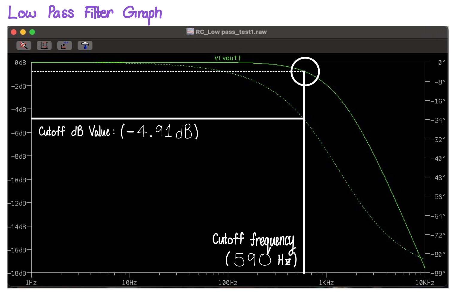
Picture 1: Low Pass Filter

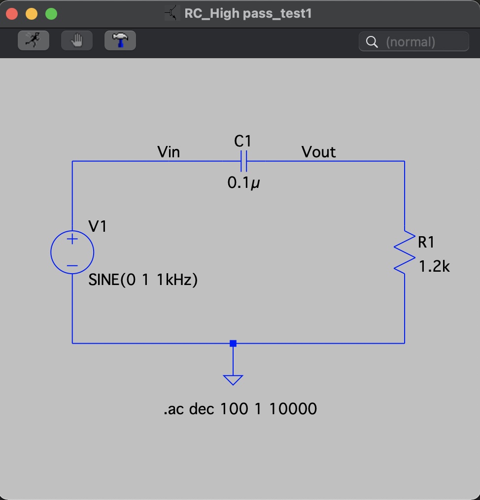
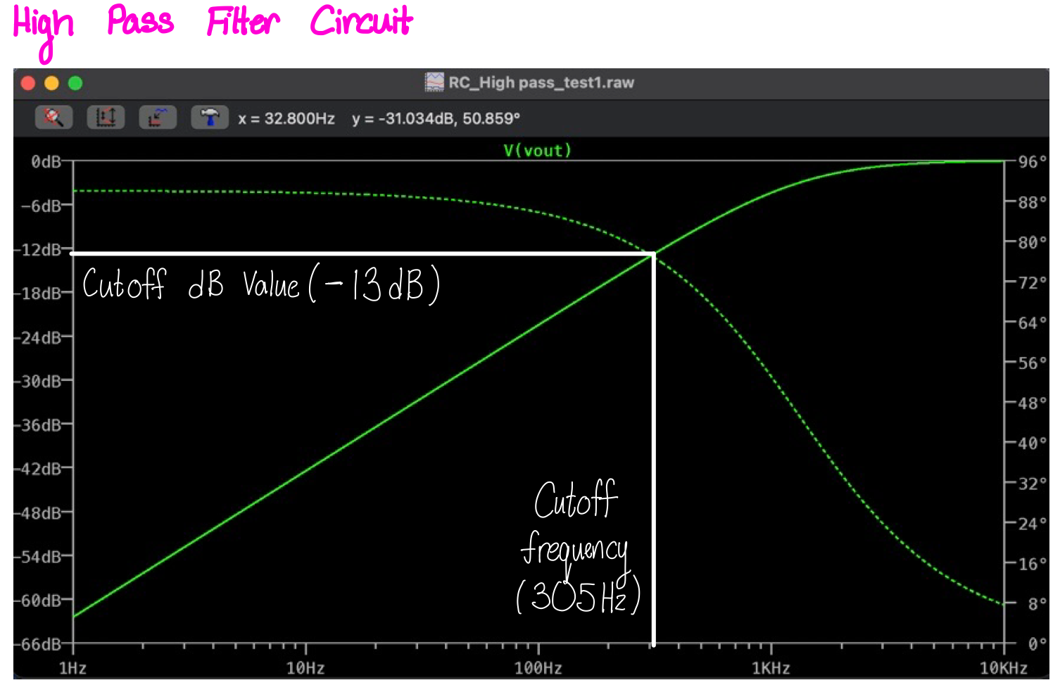
Picture 2: High Pass Filter

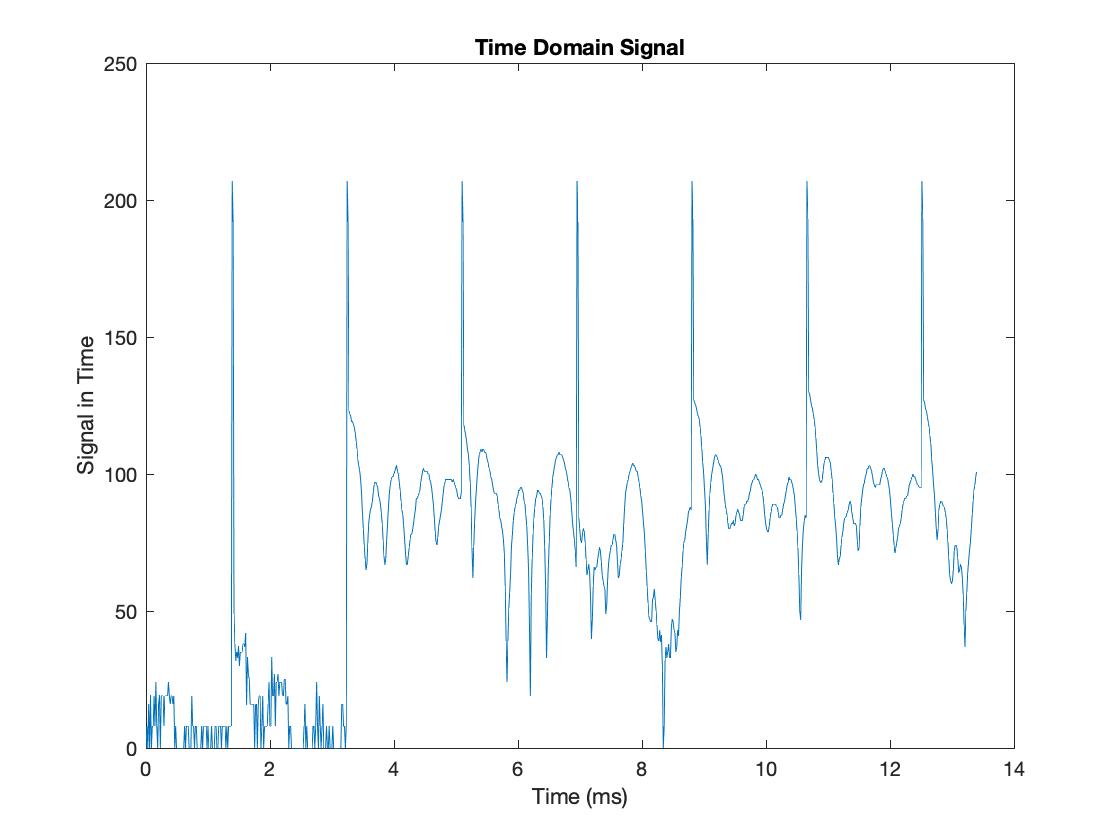
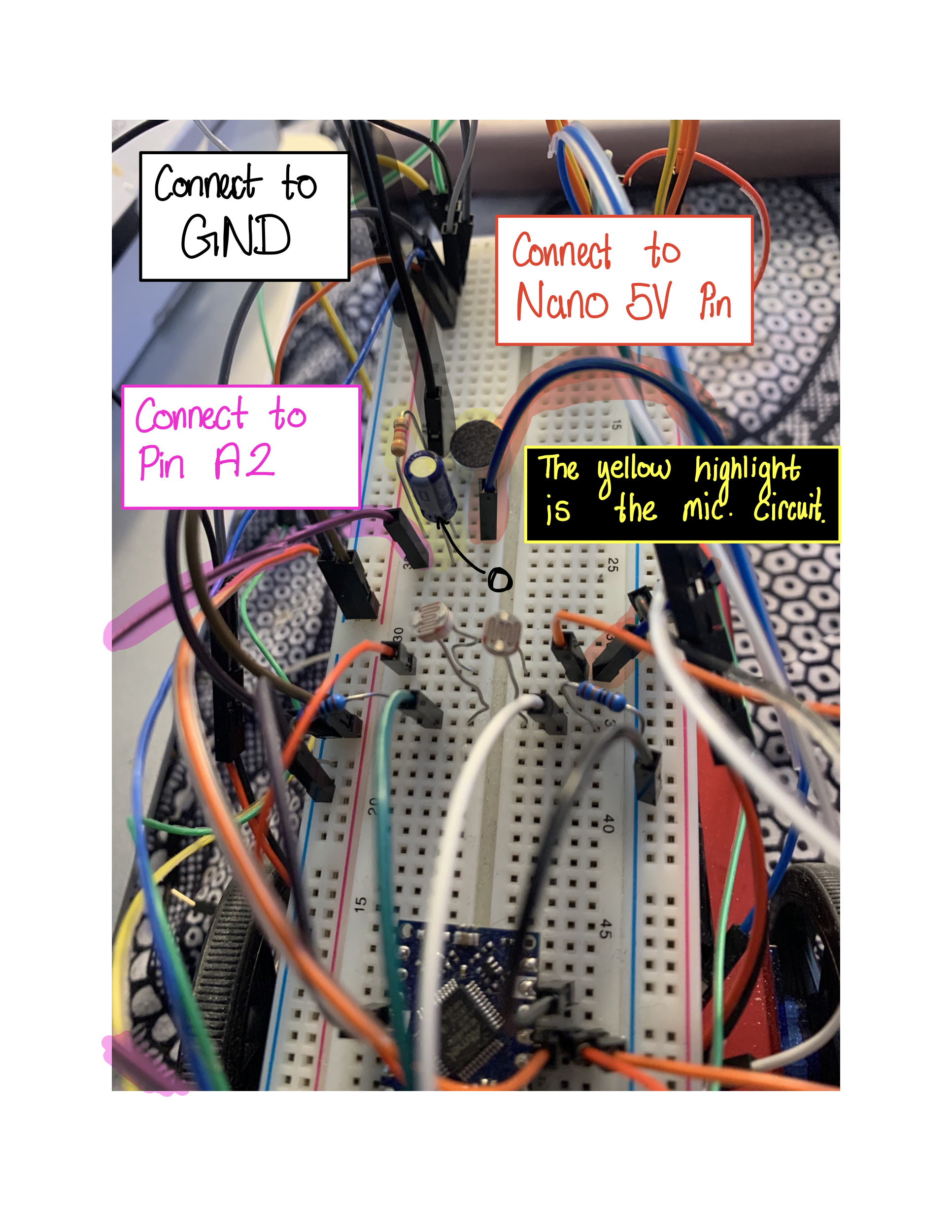
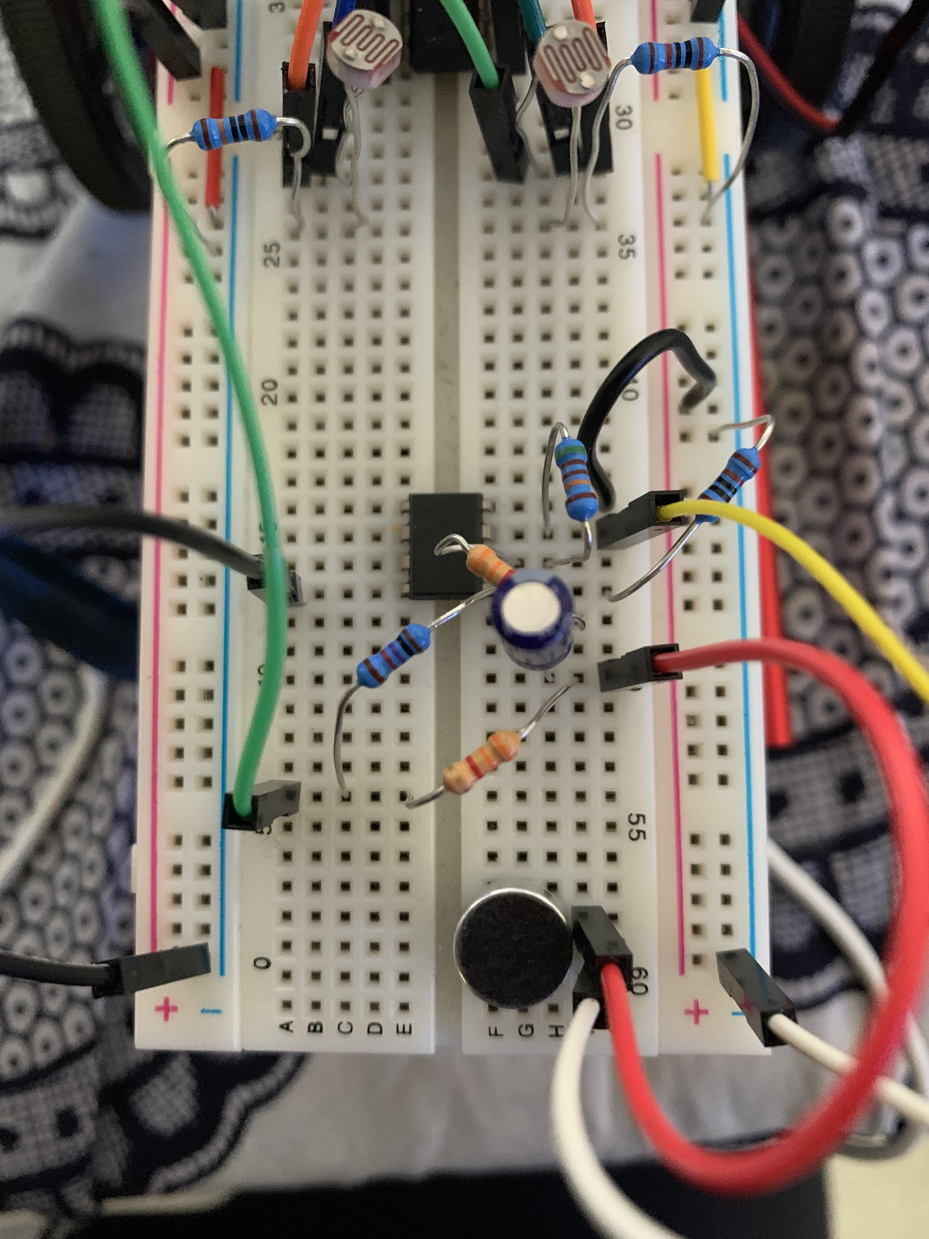
Picture 3: Basic Microphone Circuit

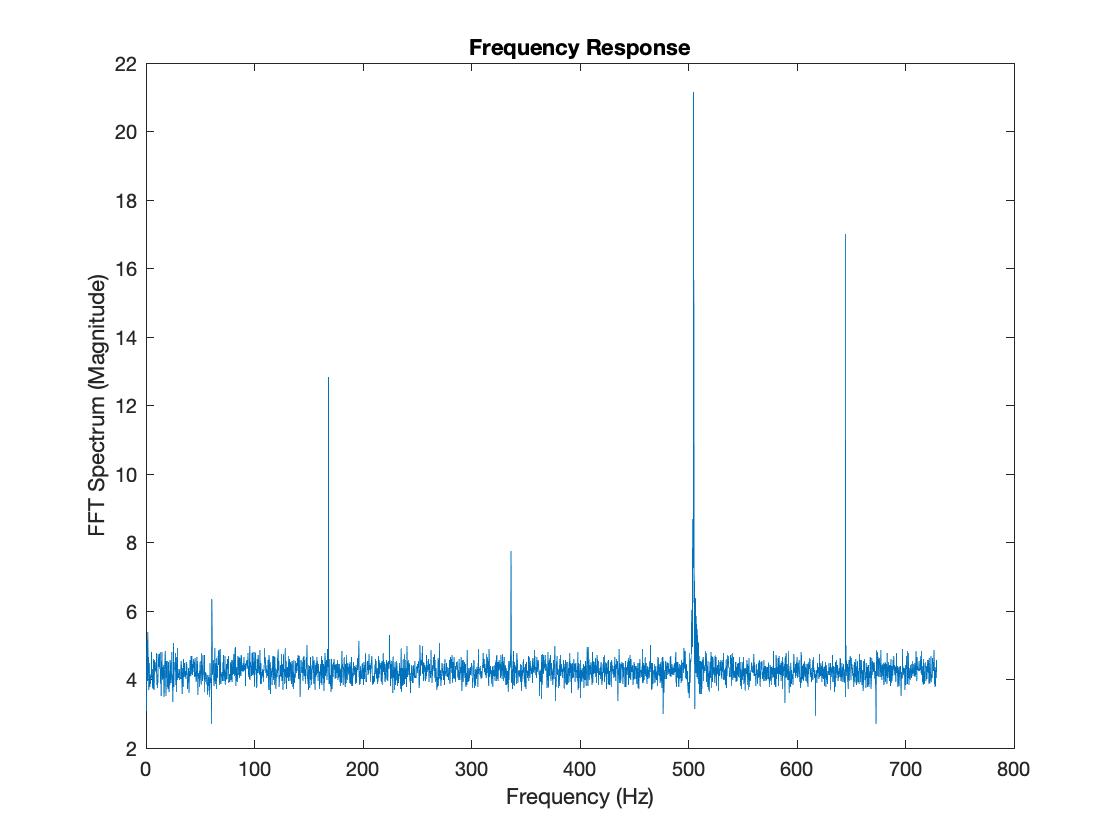
Picture 4: Graph of the data read for the Basic Microphone Circuit

Picture 5a-b: Amplified Microphone Circuit & Graph

Picture 6: Amplified Low-Pass Microphone Graph

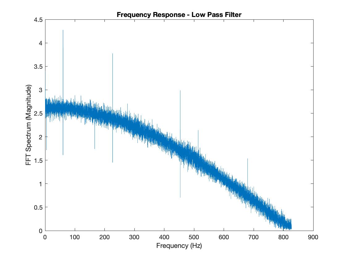
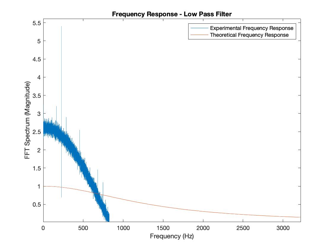
The most prominent observations that I made for the comparisons in these two graphs were that the noise level of the experimental filter response was more prominent than with the simulated filter response, and the amplitudes slightly differed. Additionally, the attenuation beyond the cut-off frequency for the experimental filter response is less gradual than that of the simulated filter response. I believe that these differences are due to the fact that the theoretical model does not account for the noise interferences from the ambient environment or the imperfections in the continuous voltage signal being fed into the experimental filter, so the data curve is smoother. Also, the volume of my speakers is adjustable, while the amplitude is set to a variable in the theoretical model.

Picture 7: Amplified High-Pass Microphone Graph

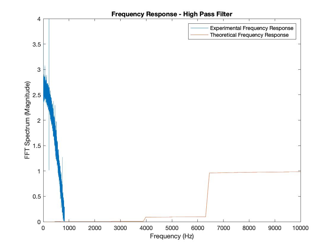
The theoretical response curve was a bit more jagged than I would have anticipated, but the general direction and trend of the theoretical response curve were not far from my expectation. Something that I noticed, similarly to the low-pass graphs, was that the noise level of the experimental filter response was more prominent than with the simulated filter response, and the amplitudes slightly differed between the two curves. There was a shaper attenuation with experimental filter response than I would have anticipated from looking at the theoretical response curve. I think that the reasoning behind these observations is similar to that of the low pass filter; the theoretical model doesn't factor in the sources of noise interferences in the responses, and the volume of my speakers is adjustable, while the amplitude is set to a variable in the theoretical model.

Picture 8: Amplified Band-Pass Microphone Graph

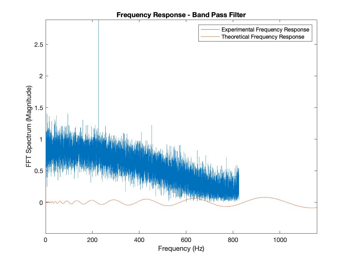
My experimental curve for the bandpass filter seems to take on the same shape as the theoretical bandpass filter, with the difference being that the experimental curve has more noise, a larger amplitude, and seems to attenuate at a different (slower) rate judging by the sector that was captured by Matlab. Other than the causes of an imperfect, unideal environment that I previously mentioned, I believe that the signal processing and timing that goes into capturing the signal for Matlab is a culprit for the differences between the theoretical bandpass filter and the experimental bandpass filter.

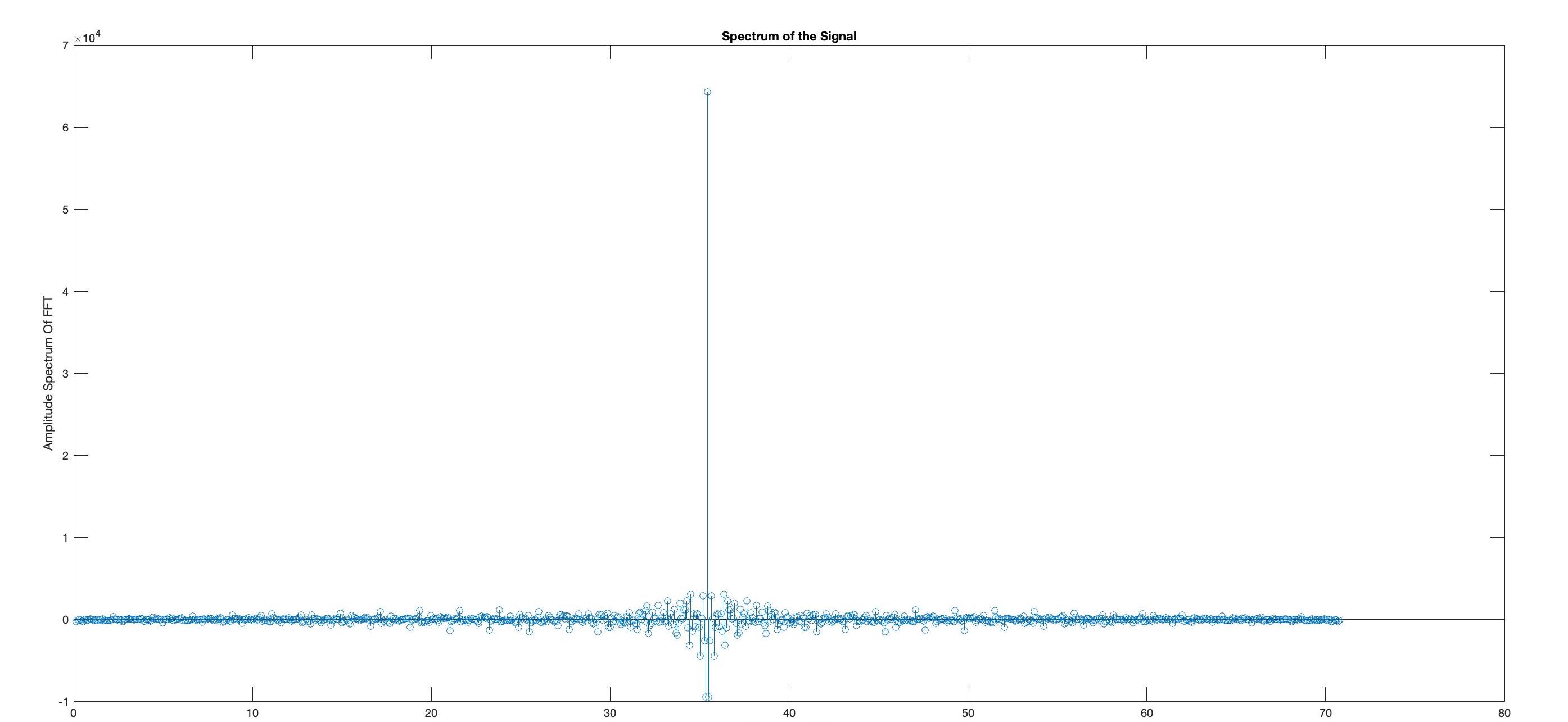
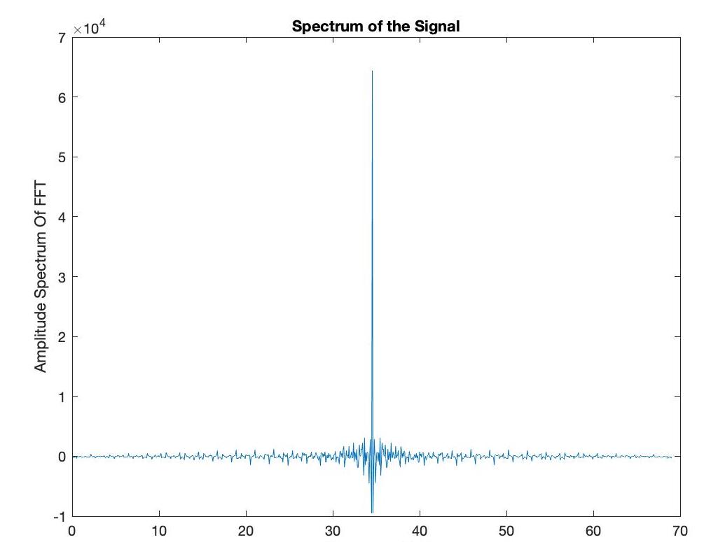
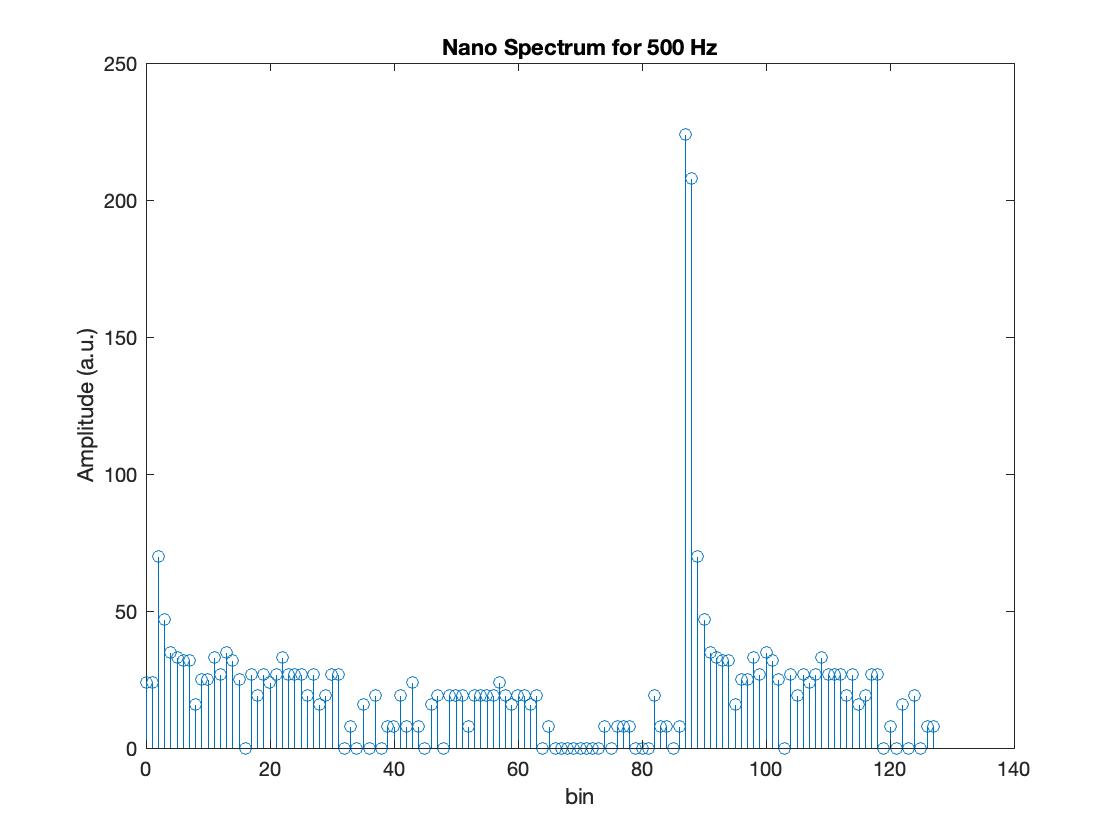
Picture 9: The spectrum obtained with the Nano for a sound frequency of 500 Hz

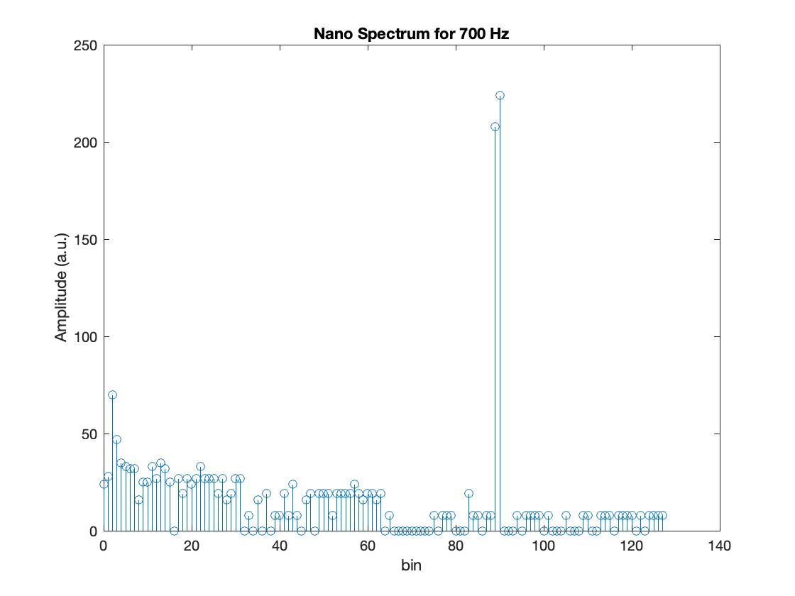
Picture 10: The spectrum obtained with the Nano for a sound frequency of 700 Hz

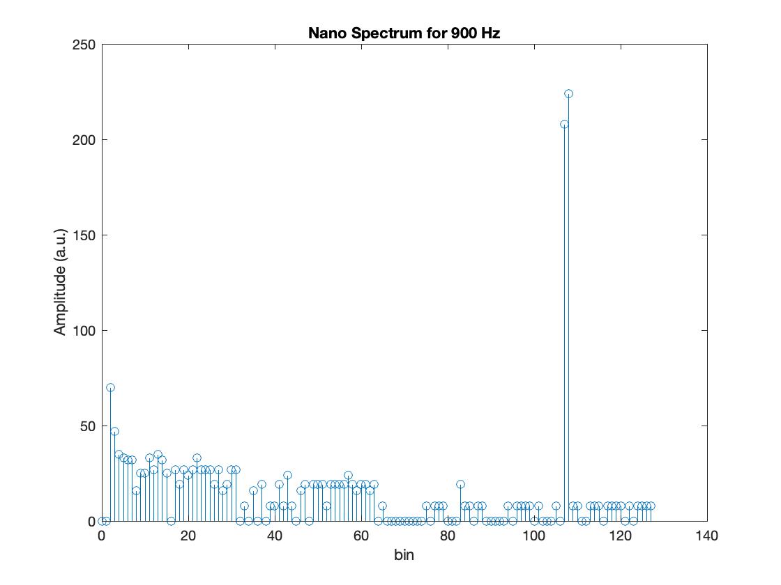
Picture 11: The spectrum obtained with the Nano for a sound frequency of 900 Hz

Summary & Takeaways

In Lab 3, my biggest takeaway was that the seemlingly more complicated method of doing things may be the most efficient and rewarding. Even though I had to redo this lab a few times to get it, I'm very glad that I did!

Next Steps

Now that I have completed this lab, my next step is to figure out how to use the bandpass filter in Lab 4.