Go To:
Home Page
Final optimization and changes for competition
To maximize our chances to succeed during the competition, we did some adjustments to Calvin prior to the competition.
Physical Design
Since Milestone 4, we made some design changes to Calvin, our robot, which include the following:
- Cut down robot width
- Adding the microphone
- Changing how we mount our treasure sensors
- Adding a team flag (a.k.a Francis’s face)
Width:
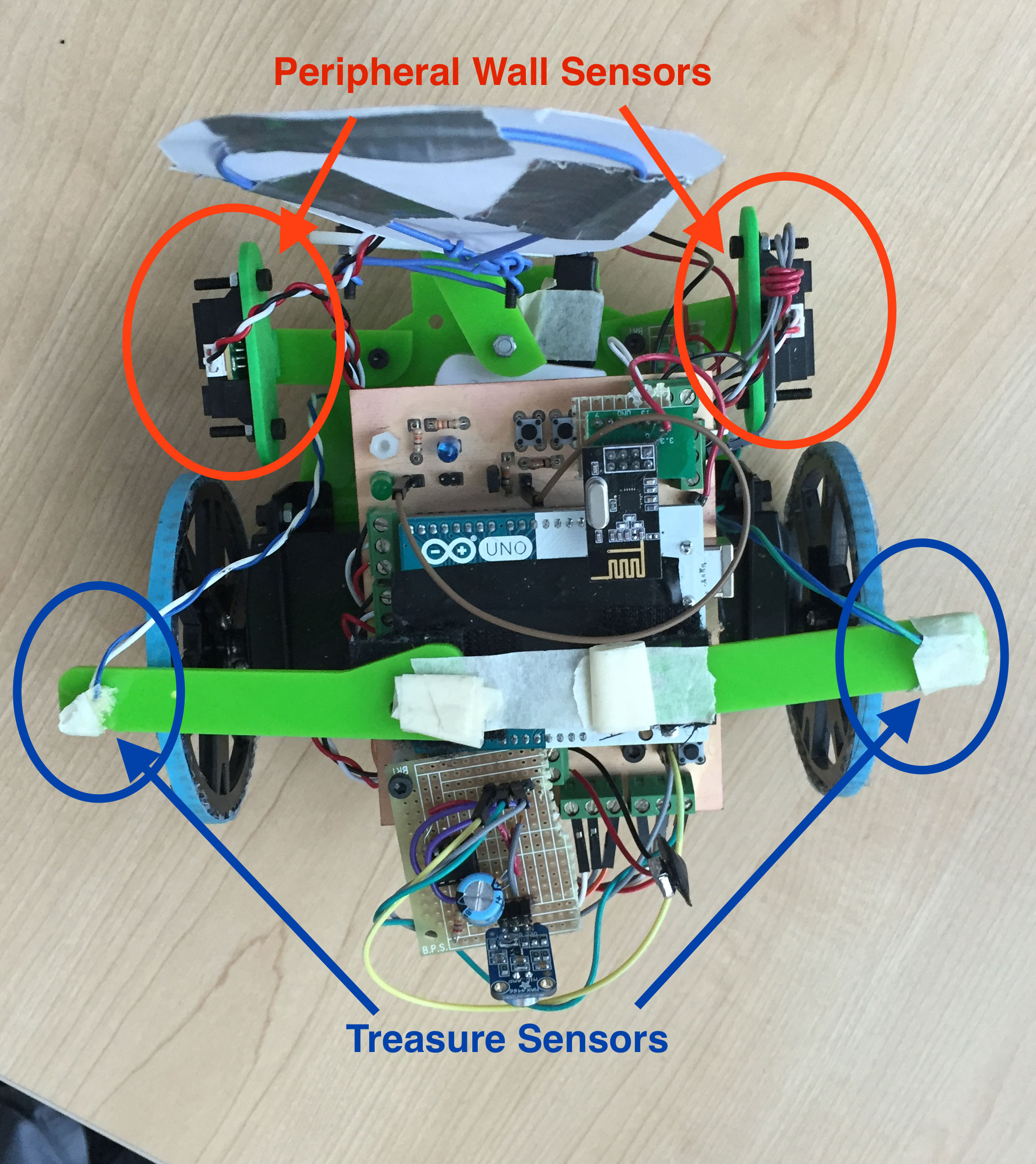
In order to make the robot smaller to ensure that it could make tighter turns, we scrapped the wings idea and moved the wall sensors in. We wanted to keep the treasure sensors as close to in line with the intersection sensor as possible to maximize its likelihood of detecting a treasure, so we taped parts of the wings to the top of the robot and hung the treasure sensors off the side over the wheels.
Microphone:
The microphone was mounted to the back end of the robot to increase it’s chances of hearing the 660 Hz tone that would be played from behind the robot. This however could have posed a problem during competition since our microphone was almost touching the back wall of the maze. If we could change our design, we would have place the microphone facing up.
Treasure Sensor Mounting:
We had to move the location of our treasure sensors since our robot was too wide with their placement in Milestone 4. We decided to break our acrylic overhangs in half and tape them to the top of our robot so that the treasure sensors hung upside down from the overhangs. The only problem with this design was that we would have to occasionally check to see if the treasure sensors were fully connected since gravity was working against us.
Opamp Circuit
In order to amplify the microphone’s signal, we decided to use a noninverting opamp circuit. We decided filtering would be pointless because the interfering signals are at the desired frequency of 660Hz. Instead, we rely on a steady 660Hz over time and if we receive that signal for long enough, we start the robot. This was robust to any talking or background noise at 660Hz. The opamp circuit is shown below: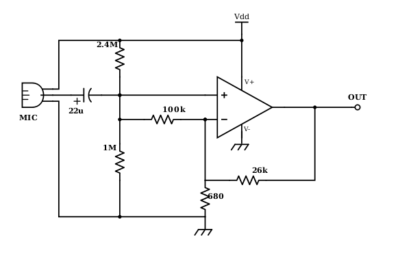
It consists of resistors in negative feedback creating a noninverting gain of approximately 40. There are many other resistors in the circuit, though, which are very important for running the circuit correctly. An opamp is designed to amplify the difference in voltage between the two input terminals. That means if there is a DC difference, this will be amplified. If this DC offset was 1V, this would be amplified by 40, so the opamp would rail the output at 5V. The 2.4Mohm and 1Mohm resistors between the power rails set a DC voltage around 2V. This is applied directly to the noninverting input and through the 100kohm resistor to the inverting input; this keeps both inputs at the same DC level. The AC signal from the microphone is coupled into the noninverting input via the capacitor, creating a signal difference between the two inputs. This signal gets amplified and returns much stronger at the output.
Speed Optimization
Upon the completion of maze exploration using the depth first search algorithm, treasure detection, and data sending to the base station Arduino, we decided to optimize Calvin to give him every opportunity to succeed during competition against the other robots.
Initially, Calvin was running at 85 for the left motor and 95 for the right motor (90 is stop). Though, we changed it such that Calvin moves 10 increments faster (75 and 105). However, despite Calvin’s previous success, the increased speed not only did not help Calvin finish the maze faster, but it made him miss turns, over turn, and even stop line following. Increasing the speed set him back significantly.
To resolve this, we first attempted to calibrate Calvin so he can line follow again at the new speed. After some debugging, we discovered that some of the delays within the line following loop had to be decreased. In the previous line following function, there was a switch statement that determined if Calvin should straight, adjust right, or adjust left for 50 millisecond; this method worked perfectly prior to the increased speed. However, the 50 millisecond adjustment at the higher speed made Calvin over correct during every iteration of the loop, thus pushing him off of the line. Once the delay was brought down to 20 millisecond, Calvin line followed perfectly again, though, this time at a faster speed.
Next, we started to debug the turns. Once an intersection is detected and treasure and wall data has been sent to the base station, Calvin either turns left, right, or continues forward. In the previous turning code, Calvin would keep turning until a line sensor hits the black line again (Left line sensor for right turns and right line sensor for left turns). However, because the turns are going a lot faster with the increased speed, using this method would make Calvin over turn significantly. Thus, we opted to use the right line sensor to stop turning for right turns and left line sensor to stop turning for left turns. In other words, Calvin would stop turning right until the right line sensor hits black, and vice versa. This way, we give Calvin a little more buffer to slow down once it hits the black line to continue to line follow.
Last, after calibrating line following and the turns to the new speed, there was one aspect that still needed to be adjusted: the get off intersection jump. After Calvin makes a turn, he moves forward just a slightly so the same intersection would not be detected again. However, at this new speed, the slight jerk sometimes misaligns Calvin’s line sensors. Therefore, once the jerk speed was hardcoded slower. All problems were solved.
After the various adjustments, we were able to make Calvin go significantly faster without sacrificing any accuracy or reliability.
FINAL CODE
Our system code consisted of 3 major parts:
- Robot Arduino Code
..* Treasure code - Communication Code
- Base Station Verilog Code
Robot Arduino Code
Our Robot arduino code was organized into an FSM that had many states to handle everything from the starting tone recognition, to treasure sensing, to maze navigation and algorithm, and even sending all the data to the base station. The FSM kept track of the state the robot was in by using a giant switch statement. Deciding when to save our data points and when to send them to the base station was a little bit tricky and was further complicated by the fact that we didn’t have a treasure sensor on the front Calvin. This means anytime there could be a treasure in front of us (anytime a wall was in front of us) we had to turn and then check for treasures again.
 switch (state)
  {
    case 1:   //STATE: Listen for Tune
     {
       ...
     }

    case 2:   //STATE: Line Following
     {
       ...
     }

    case 3:   //STATE: Intersection
     {
       ...
     }

    case 4:   //STATE: Check Treasure
     {
      //update the treasure variable here
     }
    case 5:   //STATE: Check Walls
     {
      //update the wall variable here
      //had to convert our 4 bools into a boolean to send across radio
     }

    case 6:   //STATE: Check if Complete or next node
     {
       //updated x and y variables before the algorithm because algorithm gives us NEXT location
       //ran algorithm
       //sent data to base station
       if ( done signal received )
       {
         //turn once so we can check for treasure in last location (don't have a treasure sensor on front)
         //update done variable
         //send data
       }
     }

    case 7:   //STATE: Turn Right
     {
       //check for treasure after turning
       //send data
     }

    case 8:   //STATE: Turn Left
     {
       //check for treasure after turning
       //send data
     }

    case 9:   //STATE: turnaround
     {
       //check for treasure after turning
       //send data
     }

    case 10:  //STATE: DONE SIGNAL
     {
       //we actually ended up taking care of this in others states so this just stopped our robot
       //it could have been removed
     }
  }
The rest of our robot arduino code has been discussed in other parts of the website!
Treasure code and testing
We took the code from Milestone 2 used to detect treasures and made it into a sub-function, int fft_analysis(int mux), that takes the ADMUX value of the analog pin to be read and outputs a 0, 1, 2, or 3 corresponding to the frequency of treasure detected, if any. The number corresponds to the same number that the robot sends to the basestation.
We then created a checktreasure() function that updates the value of the global variable treasure for sending data to the basestation in the following code:
/*Global variables included for reference*/
int adc_4 = 0x44;   //ADMUX value for A4
int adc_5 = 0x45;   //ADMUX value for A5
int treasure;

…

/*In main code*/
   //make sure the robot is stopped to check for treasure
   rightMotor.write(90);
   leftMotor.write(90);

   int treasure1 = fft_analysis(adc_4);  //check if treasure detected at sensor 1
   int treasure2 = fft_analysis(adc_5);  //check if treasure detected at other sensor
   treasure = max(treasure1,treasure2);  //should only detect at most treasure at one square, so the other is 0
We wrote a test file that runs the above code and turns on an LED if treasure != 0. We used this file to determine an appropriate threshold value for the fft analysis in the lab and on competition day.
When incorporating this code with the microphone code, we discovered that the ADCSRA register must be set to 0xe5 in order for the treasure fft_analysis algorithm to run correctly, but this register value interferes with the built in analogread() function. In order to fix this bug, we had to add the following code to the beginning and end of the fft_analysis() algorithm:
int init_adcsra = ADCSRA;   //save initial value of ADCSRA before function call
ADCSRA = 0xe5;   //set adc to free running mode
…
//before return statements in fft_analaysis()
ADCSRA = init_adcsra;   //restore initial value to ADCSRA
Because the robot has only 2 treasure sensors on either side, it needs to be able to check for treasures and send any new data whenever it turns. It must also turn, check for treasures, and send data one last time when it is done in case it ends with a treasure in front of it. This functionality was added to the finite state machine code by adding a checkTreasure() and sendData() line to the turn states and ensuring that the robot turns one more time when it determines it is done.
Communication Arduino Code
The next part of the system was our communcation protocal and code.
In our final iteration of the code, unlike in Lab4 in which we had to type T or R to transmit or receive, both the base station and the robot Arduino are preprogrammed to automatically send or receive data (Robot Arduino Sends; Base Station Receives).
The bits are organized as follows:
| / | / | / | / | Done | X1 | X0 | Y2 | Y1 | Y0 | W3 | W2 | W1 | W0 | T1 | T0 |
The done signal was added in bit position 11 after Lab 4 to communicate whether the robot is finished with exploring the maze. (1 means done).
*Note: For more detailed information on bit packing, please refer to Lab4 write up Lab 4: Communication Via Radio.
Arduino code data sending function
void sendData() {

  //to update new location of robot
  //putting numbers to appropriate bits
  send_x = x << 9;
  send_y = y << 6;
  send_walls = walls << 2;
  send_treasure = treasure;
  send_done = done << 11;
  message = send_x + send_y + send_walls + send_treasure + send_done;

  // First, stop listening so we can talk.
  radio.stopListening();

  unsigned long startTime = millis();
  //Serial.println("====================================");
  Serial.println("Sending Message ");
  //Serial.println(startTime);
  bool sent = 0;
  unsigned long diff = millis() - startTime;

  while (!sent && diff < TIMEOUT) { //keep sending until message is sent
    sent = radio.write(&message, sizeof(unsigned int) );
    Serial.write("message: ");
    Serial.println(message, BIN);
    if (sent) {
      Serial.println("ok...\n\r");
    }
    delay(100);
    diff = millis() - startTime;
    //Serial.println(diff);
  }

  // Now, continue listening
  radio.startListening();
  }
Once the base station Arduino receives the signal, it will transmit the received information via the SPI protocol to the FPGA. An important thing to note is that once the base station receives the bit package, it MUST turn off the radio (by writing port 10 high) before sending the FPGA the signal via SPI. Since the Radio module also uses the SPI bus, not turning off the radio while writing to the FPGA will cause lots of collisions.
Below is a snippet of the base station Arduino code that we used in the final competition for receiving from the robot and sending to the FPGA.
Receiver Side Code Snippet
 // if there is data ready
    if ( radio.available() )
    {
      // Dump the payloads until we've gotten everything
      bool done = false;
      while (!done)
      {
        // Fetch the payload.
        Serial.println("============");
        done = radio.read(&got_message, sizeof(unsigned int) );
        printf("Got message = b" );
        Serial.println(got_message,BIN);

      // Delay just a little bit to let the other unit
      // make the transition to receiver
      delay(20);
      }

      // First, stop listening so we can talk
      radio.stopListening();
      // Send the final one back.
      radio.write(&got_message, sizeof(unsigned int) );
      printf("Sent response.\n\r");

      //SPI Code
        digitalWrite(10,HIGH);  //unselects radio MOSI
        digitalWrite(vgaCS,HIGH);   //tells VGA to read
        SPI.beginTransaction(SPISettings(1000000,MSBFIRST,SPI_MODE0));
        SPI.transfer16(got_message);
        SPI.endTransaction();
        digitalWrite(10,LOW);
        digitalWrite(vgaCS,LOW);
        delay(500);

      prev_message = got_message;

      // Now, resume listening so we catch the next packets.
        radio.startListening();
Field Programmable Gate Array (FPGA)
The final part was the FPGA. This was done in verilog which was extremely finicky to use. The FPGA handled the reciever side of the SPI communication, the display, and even played the done signal using a sine table to play a sine wave at different frequencies. The SPI and done signal did not change from milestone 4 at all so you can look there for the full breakdown of it. There were a few minor changes to the FPGA display though. We decided to change the color scheme to something a little bit more pleasant on the eyes.
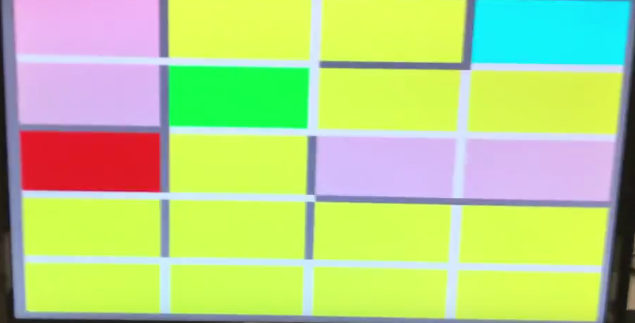
As you can see we changed untraveled to rosy brown, traveled to a yellow, a wall to dark gray, potential wall spot (without a wall) to white, and untravelable to black. The untravelables change to black once the done signal is received. Changing these was fairly straight forward, assuming our robot algorithm could complete the maze. Any location that was untraveled after the done signal was received had to be blocked off by walls or else it would have been traveled to. While doing these we also decided that we would change the potential wall locations INSIDE of the untravelable zone to black also. This was strictly an aesthetic choice. Along with that we changed all traveled to locations to a lighter yellow to display a done signal (in ase there is not untravelable zone). Finally, we had to make to our verilog code was accounting for the last position having a treasure in front of it. Since we have to turn to check for a treasure, our old code was ignoring the last signal since we only updated anything if the current and prev locations were different. To take into consideration this corner case we had to update it to this:
if (reset == 1) begin
  //this changes everything to the starting colors
  //i.e. locations to untraveled, outer walls to gray, inner walls to white
end
else if (X_CURR == X_PREV && Y_CURR == Y_PREV && treasure != 0) begin
  //had to add this to check for the corner case
  //we also added the check for the done signal here (same as below)
end
else if (!(X_CURR == X_PREV && Y_CURR == Y_PREV)) begin
  //this would have filtered out the corner case
end
else if (done == 1) begin

if (grid_color[0][0] == unvisited) begin  //check if its untraveled
  grid_color[0][0] = cant_do_it;  //change it to untravelable
end
if (grid_color[0][0] == visited) begin  //check if its untraveled
  grid_color[0][0] = no_wall;  //change it to untravelable
end
if (grid_color[0][1] == unvisited) begin
  grid_color[0][1] = cant_do_it;
end
if (grid_color[0][1] == visited) begin  //check if its untraveled
  grid_color[0][1] = no_wall;  //change it to untravelable
end
... //check all locations to update them to their done state colors

//this code changes the walls in the untravelable zones
//anytime a wall is between any two untravelable locations it should turn black

if (grid_color[0][0] == cant_do_it && grid_color[0][1] == cant_do_it) begin
  grid_color[0][6] = cant_do_it;
end
if (grid_color[0][1] == cant_do_it && grid_color[0][2] == cant_do_it) begin
  grid_color[0][7] = cant_do_it;
end
... //check all possible combinations
Here is an example of our VGA display:
Go To:
Home Page
Algorithm
We are the runner-up in the Fall 2017 competition. You must be thinking that we have a very efficient and complex algorithm. We are sorry to disappoint you, but we do not. We showed up to the final competition with good old, very basic Depth-First-Search (DFS) algorithm. We were not very proud of the simplicity of this algorithm, but we were confident about the stability, safety, and consistency of Calvin’s performance with the simple DFS. And that is how we won the second place in the final competition.
Let us briefly summarize why the simple DFS is not a bad choice at all.
- DFS is ideal for forward exploration. Given the high cost of turning, DFS is much more suitable than Breadth-First Search in the forward exploration.
- Our competition takes place on a grid of 5 by 4 size. The fact that there are only 20 grids makes the room for improvements by algorithm alone smaller than we think.
- Simple DFS is very memory-efficient. Other than trivial memory assignments to variables, DFS uses very small number of helper functions, and all it needs are, 1. linear array size of 20, each element containing 16 bits—total of 40 bytes, which hold all necessary information the algorithm needs to lead the path, and 2. stack, which will most likely not use more than 20 bytes of memory.
- DFS without modification is infallible. In other words, no matter how slow it might be, we can trust that Calvin will finish the maze and stop at the right time (as soon as all grids were explored), not fearing the possibility of going through infinite loops and never finishing the maze (please wait until we explain what we mean by this!).
As long as wall sensors are consistent, we were confident that Calvin would finish the maze exploration—the biggest grading factor in the final competition. We decided to focus our limited time resources on making sure that the hardware components, particularly line sensors and wall sensors, are absolutely consistent. However, our story with the algorithm does not end here prematurely. Before sealing our final code with Calvin before the day of final competition, we took a long journey of attempting to find more efficient and safe algorithm, and on this page, we would like to share with you our learning, in hopes of helping you making a right choice and achieving both safe and fast algorithm.
In Milestone 3, we provided a detailed explanation of our optimization with the backtracking algorithm. To give you a brief recap, we attempted to apply localized greedy algorithm during the backtracking process. DFS can be separated into two regimes: one forward-exploration while adding neighboring grids to the stack as target grids for later exploration, and the other backtracking to the next remote target grid once it is either in the corner surrounded by three walls or all neighboring grids have already been explored.
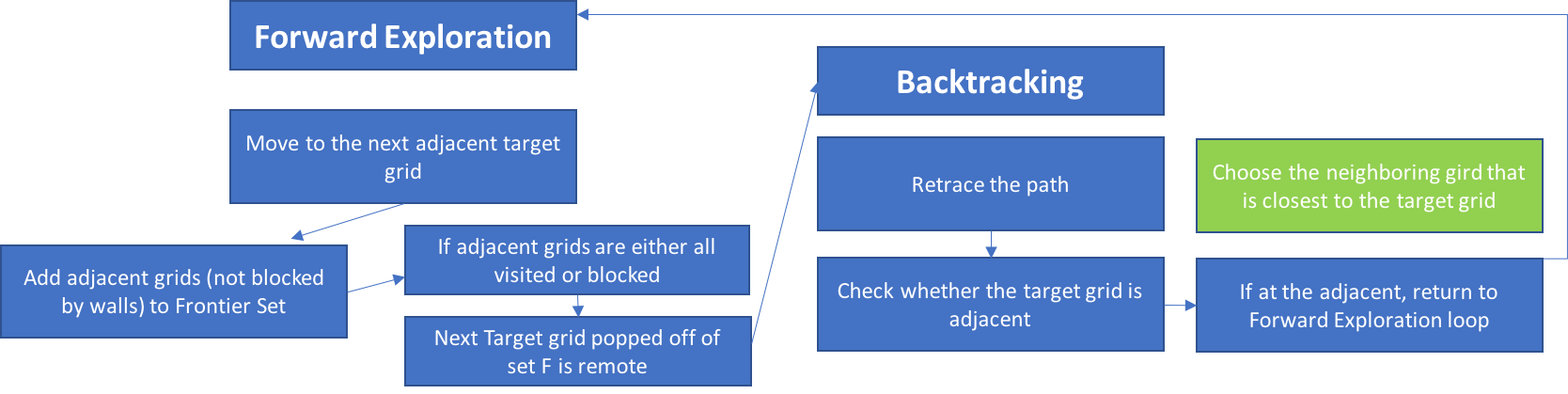
The frontier set is maintained by a stack, and DFS’s weakness becomes apparent when the next target in the frontier set is remote from the current location of the robot. Unless we can draw an exact path, hopefully the shortest one, and provide it, all the robot can do is to retrace its step, until it reaches the target. This retracing is enabled by storing the back-pointer for each grid in the linear array (please refer to Milestone 3 for detailed array data structure). Quite obviously, many of retracing steps are wasteful.
Below is the actual maze that was used in the final competition, in which our Calvin is heading toward the final target grid.
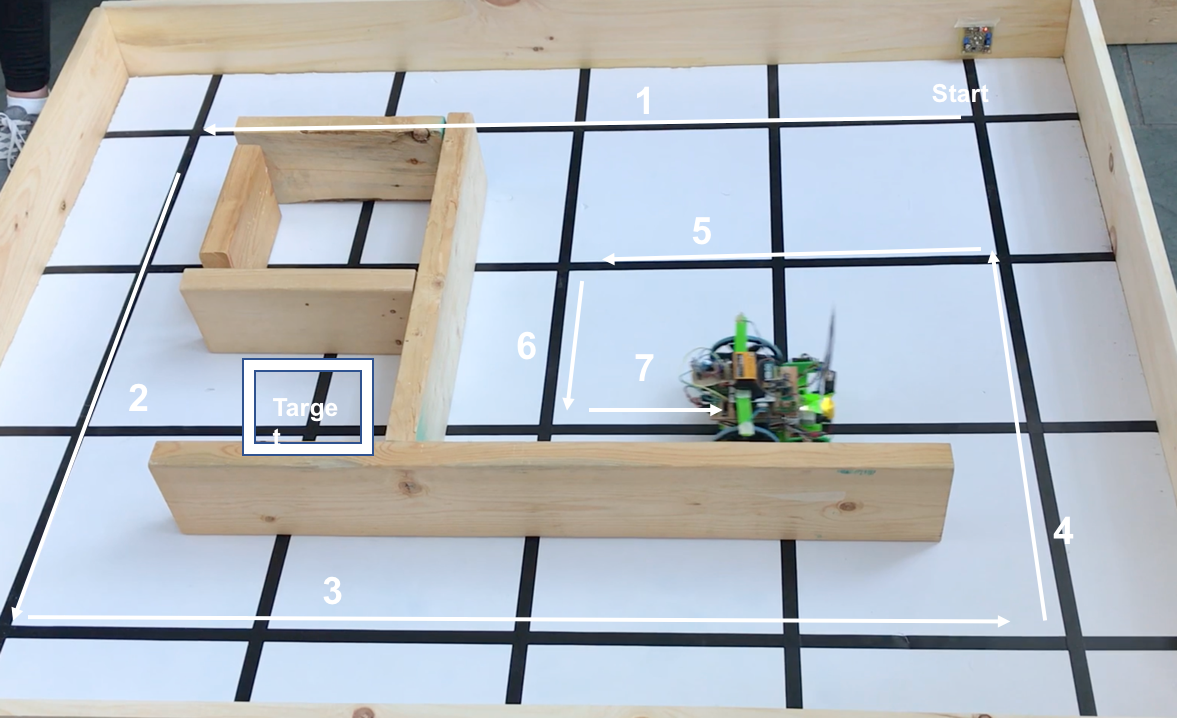
Isn’t DFS so efficient when the robot is only forward-exploring? Calvin was able to explore pretty much all of the maze with the least number of turning and, probably, the least memory usage; this is why DFS is our favorite algorithm. Now that the target is at the remote place (and incidentally, this is the last grid Calvin has to explore!), all Calvin has to do is go forward one step, turn right, keep heading straight until it sees the wall, turn right, and just one more step. Easy, right? But, the next picture shows Calvin acting unintelligently.
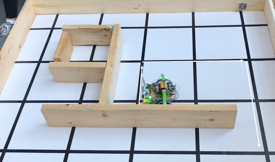
Calvin is turning back! It is following the back-pointers, and retracing the path 4-5-6 in the order of 6-5-4. Because of this process, Calvin had to travel five more grids than what would have been the fastest route, including four turnings.
This kind of inefficiency was very obvious from the beginning when we first tried out the algorithm in Java-based simulation. And what we came up with was to designate certain grids as “special” by assigning 1 to ‘isSpecial’ bit (we fortunately had 1 bit leftover from 16 bits). At the special grids, the algorithm does not merely resort to the back-pointer, but compare distances from adjacent neighbor (not blocked by walls) to the remote target (Manhattan distance: difference in x-coordinate + difference in y-coordinate). And, if two neighbors generate the same distances, we prioritize the one on north of the current direction the robot faces.
In the example above, at the end of path 7, there are three neighboring nodes. Unless there is only one open neighbor, we do not choose the previous grid. And thus, Calvin would have moved straight (both forward and right grid have Manhattan distance of three), and next follow its back-pointer path of 4-3-2 to arrive at the target in the shortest path.
Wait. Why do we not add the previous grid? Technically, the grid Calvin was on before is the closest to the target out of all three available neighbors. And, in our very earlier version of optimization, we included all neighbors as a possible candidate of local greedy choice. We started excluding it, in an attempt to avoid the pitfall of greedy algorithm.
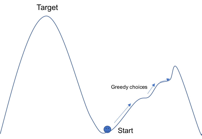
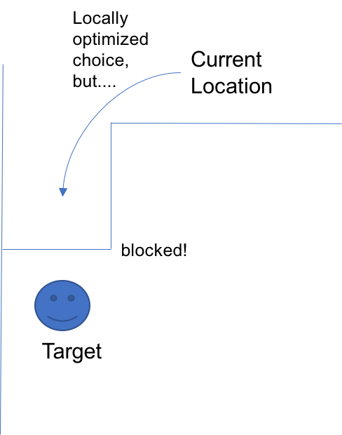
Take a look at this mountain. From the bottom well, we have to climb up to the Target. At each local point, from the onset, we make an optimum choice by climbing up. As we climb up, however, we are not getting close to the target; in fact, we travel to the opposite way. This is why localized greedy algorithm fails in many cases. Our utilization of Manhattan distance and moving to the neighboring grid closest to the target grid is localized optimization without taking the full picture into account. Yes, the next grid our robot moves to might be closer to the target, but what if the way it is heading toward is later completely blocked by the walls? (This is why we decided to exclude the grid behind when choosing neighbor for a ‘special’ grid).
This is why there are so many complete shortest-path finding algorithms, such as Dijkstra’s algorithm, A* search algorithm, and Prim’s algorithm. What Dijkstra’s algorithm does, for example, is pre-travel all possible routes to the remote target, before actually moving onto the next grid. The algorithm pre-travels all routes that look deceptively closer in local scale, and take out all of those not ultimately leading to the target. It is, therefore, guaranteed to find the real and global shortest path.
The obvious disadvantages in using Dijkstra’s algorithm is relatively large amounts of memory usage. We thought we could dispense with complex algorithms and instead use 1bit left-over from the main array that would be otherwise left unused. Because the robot moves in the second-timescale, the computation time-complexity was not our concern at all. Instead of borrowing a huge chunk of memory in finding and storing the shortest path, why not first move the robot, and whenever necessary, do simple calculations and make a locally optimal choice?
But, as we tried out in various types of mazes, complications were developed. Firstly, how do we know which grid to mark as “isSpecial”? Most of time, DFS’s default back-tracking mechanism coincides with the shortest-path. And so, we first decided to mark the starting grid of the path to the remote target grid as special, because as long as we choose the right neighboring grid as the first step in the back-tracking path, we thought the rest of DFS’s back-pointers will lead to fairly short path toward the target, if not shorter than the actual shortest-path.
Basically, the more grids we designate as ‘Special,’ the more our optimization resembles Breadth-First Search or Dijkstra’s in back-tracking, in a way all of them attempt to find the shortest path in every grid. Except, our way of optimization can never be guaranteed of safety, because we already start move before knowing that the path is in fact ultimately open to the target grid.
As we tried the algorithm on different mazes, we found corner cases, where the robot falls into pitfall, and continue to go back and forth indefinitely. More importantly, we realized that relying on both the localized greedy algorithm and general back-pointers is dangerous. On the maze above, it is fortunate that once the robot moves straight, it can make a smooth transition to following the back-pointers of path 4-3-2. However, what if the path 4 was in opposite way? What if the back-pointers build up the path opposite to the ultimate target grid? The algorithm fails in these corner cases, too, and at this point, we realized we cannot guarantee the consistency of the algorithm, and fell back to the plain DFS algorithm. (We still added the code with the optimized back-tracking algorithm on our final code folder!)