Lab 3: Filtering and FFT
Objectives:
- Implement ADC conversion.
- Use interrupts to control the sampling frequency of the ADC signal.
- Build a microphone circuit.
- Build an amplifier circuit.
- Build a high pass filter.
- Use FFT to identify frequencies using Matlab.
- Use FFT to identify frequencies on the Arduino.
Materials:
- 1 Robot and circuits from last lab
- 1 Microphone
- 1 LM358 op-amp
- 3 100 k𝛺 resistors
- 1 4.02 k𝛺 resistor
- 1 75 k𝛺 resistor
- 1 49.9 𝛺 resistor
- 1 2.7 k𝛺 resistor
- 1 100 pF capacitor
- 1 0.22 𝜇F capacitor
- 2 2.2 𝜇F capacitors
- 1 0.1 𝜇F capacitor
- Jumper wires
Simulating Filters:
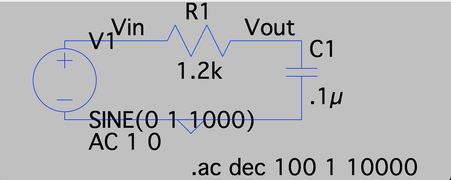
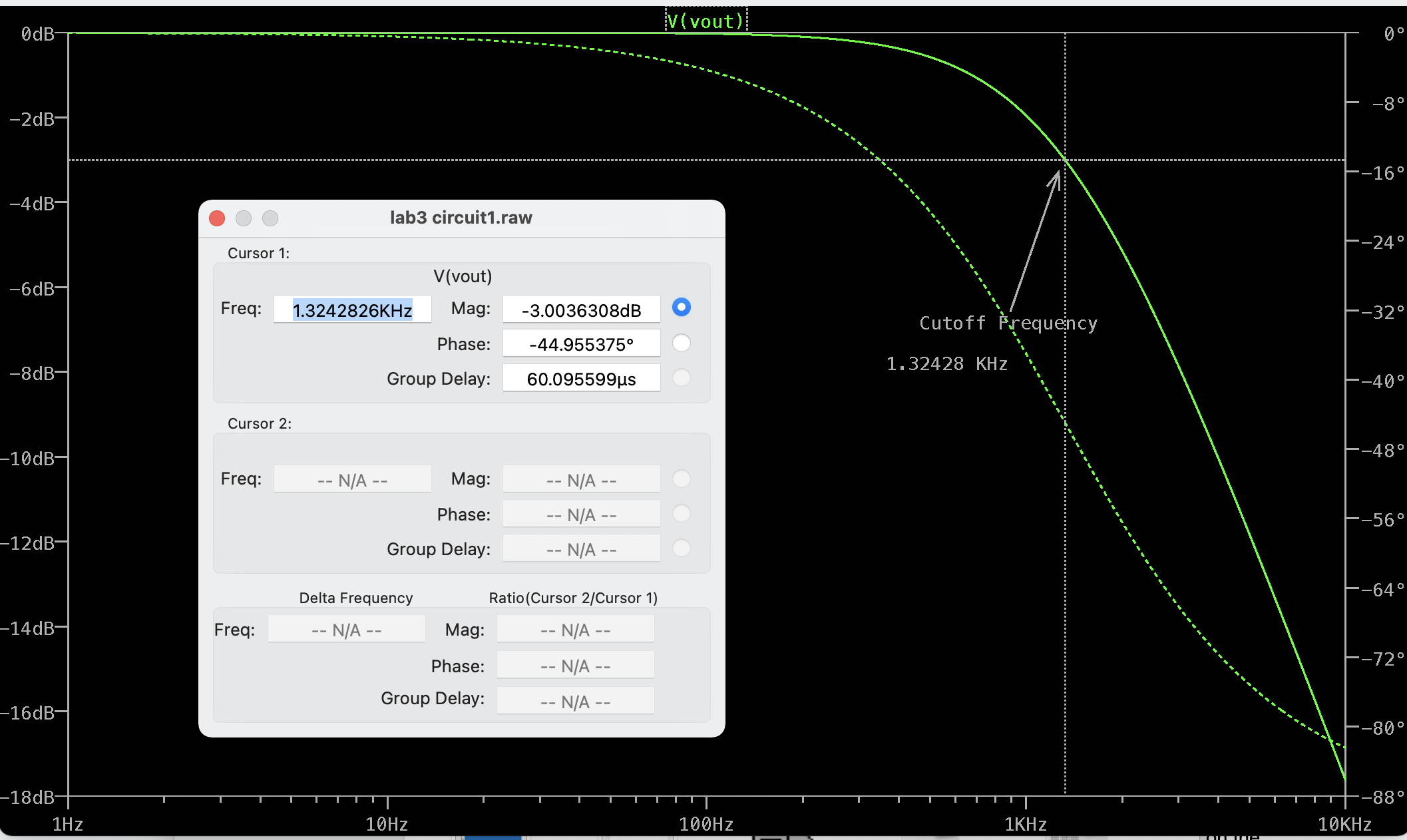
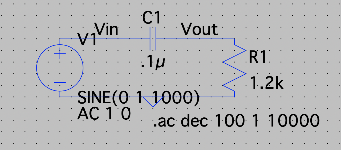
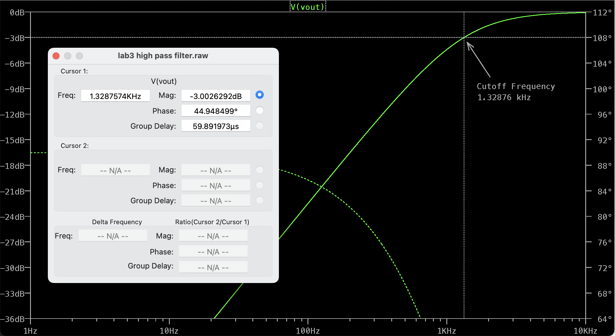
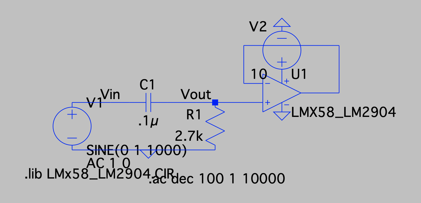
Before we began working on our circuits, we first simulated some filters in LTSpice. We simulated both a high pass and a low pass filter. The first image below is the low pass filter. We simulated a frequency sweep from 1Hz to 10kHz. The transfer function generated can be seen below the circuit. We next simulated a high pass filter, as seen in the third image. Again, we simulated a frequency sweep, and the transfer function is shown in the fourth image below. Finally, we added an op-amp to simulate the filter we built for the lab. This circuit can be seen in the fifth image. This was again simulated; the transfer function for this circuit is shown in the filter section of this page.
The Microphone Circuit:
We next implemented the microphone circuit. This circuit was fairly simple. We use a 4.02 k𝛺 resistor connected to the 5V rail to properly bias the microphone. We then used a 0.22 𝜇F capacitor to filter out the DC component of the voltage generated by the microphone. We connected this output to an analog pin on the Arduino and used ADC to convert the signal into a digital signal we could process. The circuit can be seen below. We then sent the data through the serial port to a computer running Matlab, which ran a FFT and produced a spectrum. The spectrum can be seen in the second image below. In reality, the unamplified circuit response is very weak. While the produced spectrum looks good, we had to hold a loud phone playing a 500 Hz tone directly next to the microphone to get this response. If we just played the sound off a computer nearby, there would be almost no peak at all.


The Amplifier:
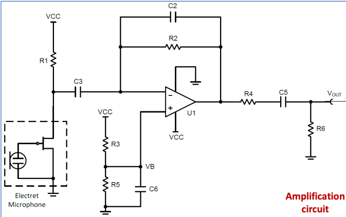
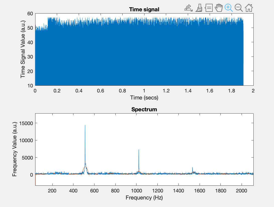
We next built an amplifier circuit so we would get a stronger signal than the microphone alone could provide. A diagram of the circuit can be seen below, and the actual implementation can be seen in the second image below. After implementing the circuit, the response measured by the Arduino was much stronger. This can be seen in the third image below, which is a Matlab plot of the FFT of the data recorded. This circuit was very difficult to get right. Often small tweaks would result in a very poor signal. It was essential to ensure that all the connections were solid. Again, the image shows the result after holding a phone close to the microphone, as that resulted in the clearest signals.

The Filter:
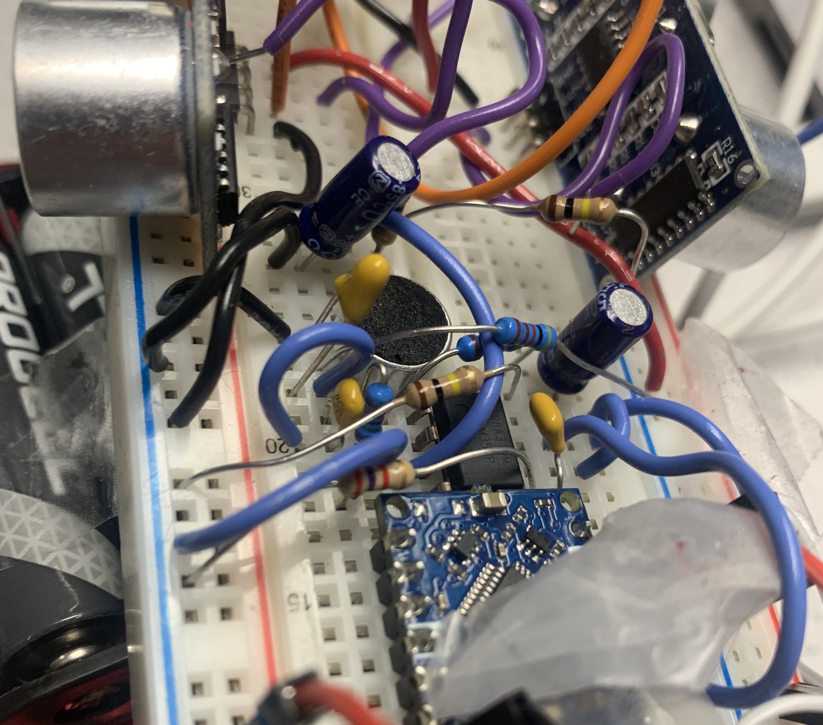
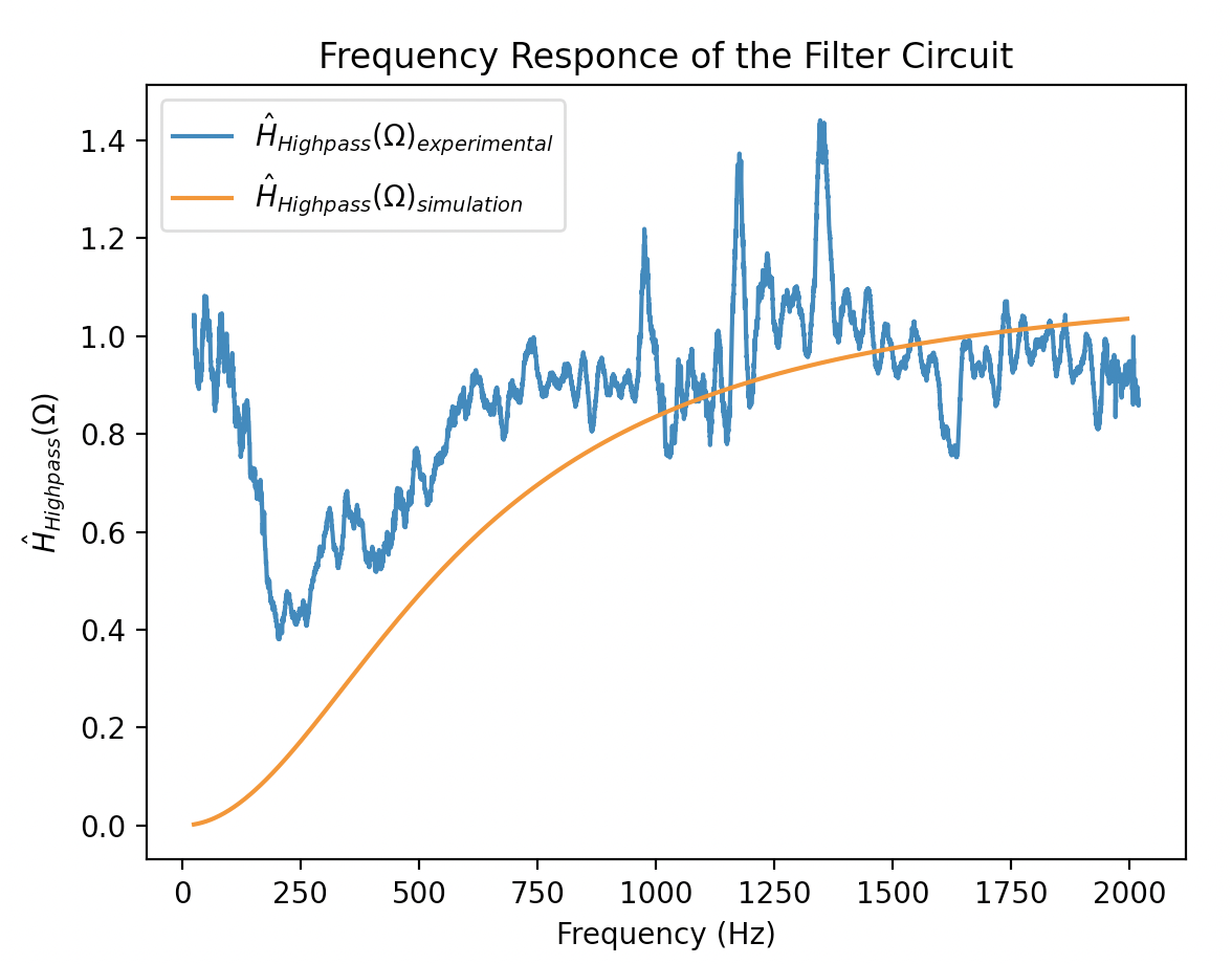
We next build the high pass filter we had previously simulated. We connected the filter to the output of the amplifier circuit. We chose to use a 2.7 k𝛺 resistor and a 0.1 𝜇F capacitor so that our cutoff frequency would be just over 500 Hz. The expected cutoff frequency was 589.46 Hz. This circuit can be seen in the image below. We then ran a frequency sweep from 100 - 2000 Hz to determine the frequency response. We measured the voltage both before and after the filter and divided the results to produce a transfer function. This transfer function can be seen in the second image below. Also pictured is the transfer function from the simulated circuit. Both transfer functions show a similar shape, but the experimental data reaches its cutoff frequency earlier. This may be due to imprecision in the resistance and capacitance of the resistor and capacitor. Additionally, the experimental data is very noisy, as there was background noise in the room, and the circuit is not incredibly precise.
FFT through Matlab:
To gather frequency data, we initially sent the data over the USB to a computer running Matlab. We used a Matlab program to read the data and perform a FFT on the data, producing a spectrum. All the above frequency data was collected in this way. Testing with Matlab allowed us to ensure that our circuit was performing correctly, as we could see what the frequency measured was.
FFT through Arduino:
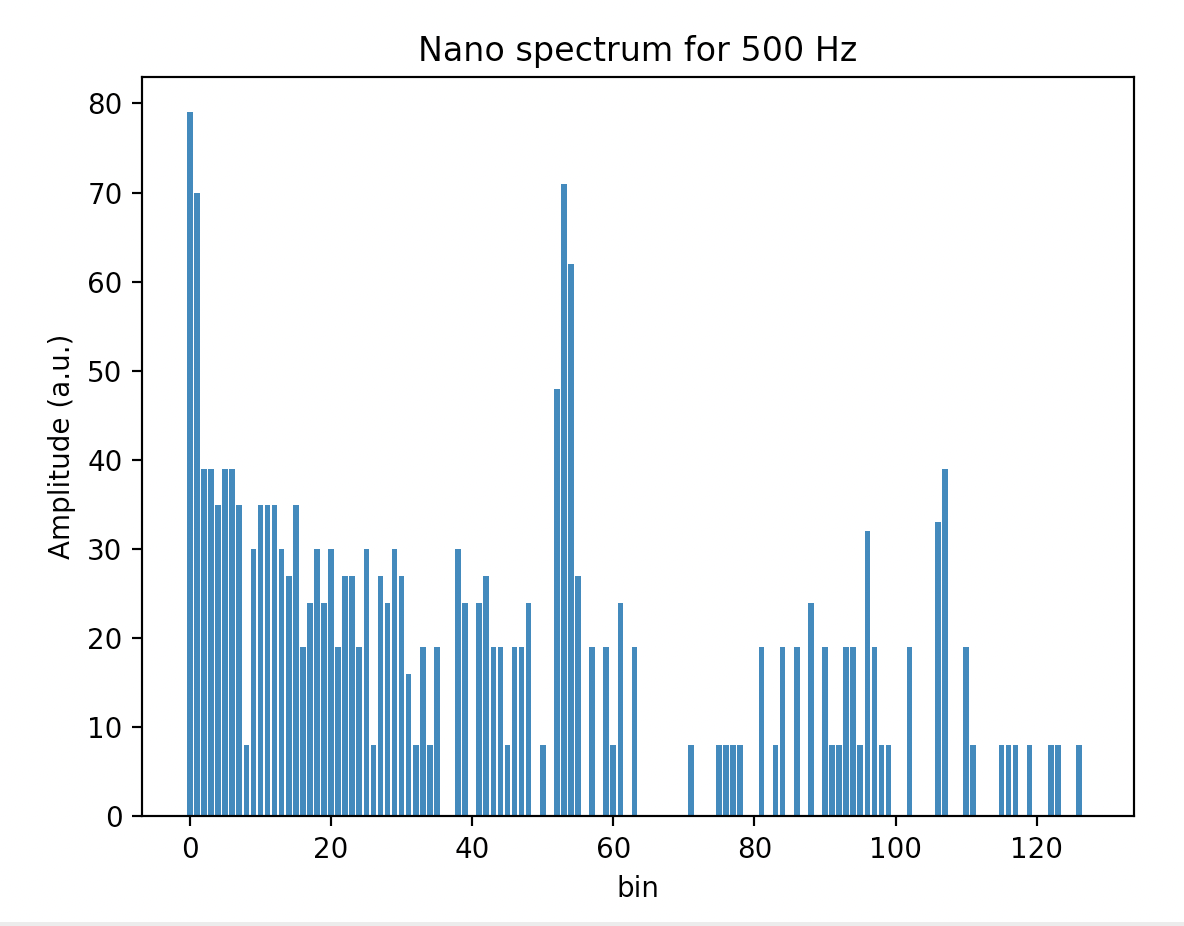
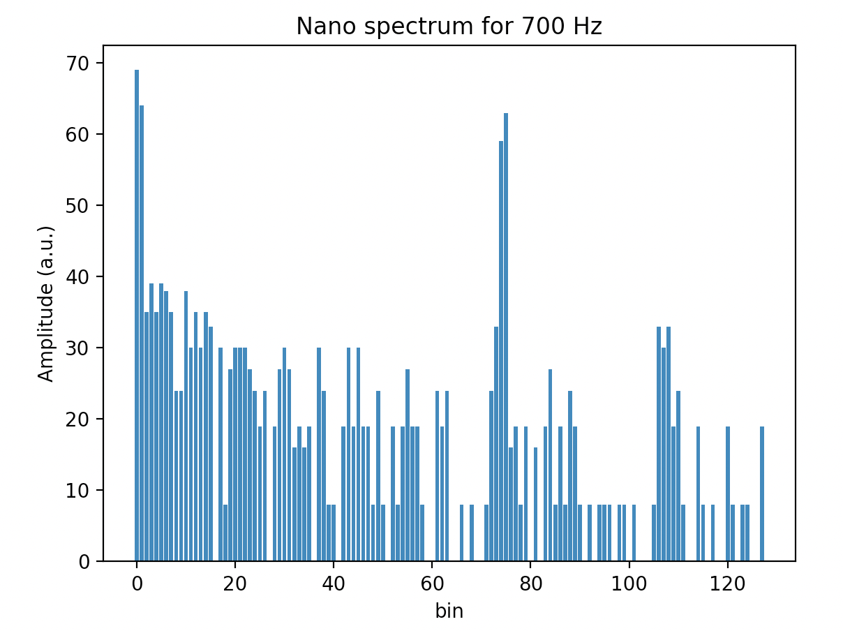
We later switched to performing the FFT directly on the Arduino, using a library. This is necessary because we will need to identify specific frequencies during the final challenge. We will not have a computer connected to the Arduino during this time, so all of the calculations must be done on the microcontroller. The disadvantage of using the Arduino to perform FFT is that the data is not as informative. Instead of knowing the frequency of each peak, we only know what bin it falls in. This can be mapped to frequency, but it is much less precise than the FFT from Matlab. The spectrums from measuring 500 Hz, 700 Hz, and 900 Hz can be seen below. The primary peak is clearly shifting to different bins as the frequency increases. Again, this data was recorded with a loud phone playing the frequency close to the microphone, as a loud signal was required to get a clear response.
