Lab 3

Materials

• 1 x SparkFun RedBoard Artemis Nano
• 1 x USB Cable
• 2 x 4m TOF Sensor
• 1 x 9DOF IMU
• 1 x Qwiic Connector
• Ruler

Prelab

I2C Address

The sensors used in this lab work with I2C communication protocol and thu need a reference address for data transaction for communicating with the Artemis. After Referencing the sensor's respective datasheet, we found the I2C address of the TOF sensors were 0x52 and the address of the IMU to 0x68 or 0x69 (More on this later)

Communication Method

Since we are working with two identical ToF sensors, we run into a problem of communicating independently as the I2C addresses are the same. To solve this issue, I decided that in order to etablish distinguishable communication link between the two sensors, I would programatically change their I2C addresses. The benefits of doing this is that you extract real time data simultaneously between the two sensors without having to do a digital shutdown of one of the sensors. Additionally, it would limit delays associated with data propagation if we maintain different addresses rather than executing shutdowns everytime, we want to communicate to one of the sensors. However, I must admit that using a digital shutdown method might be more energy efficient as the current consumption of the sensor drops from a 16mA during nominal use to 5uA while Hardware standby. Furthermore, depending on the task you're trying to achieve you might not need the second sensor and thus, the digital shutdown method might come in handy.

Sensor Placements

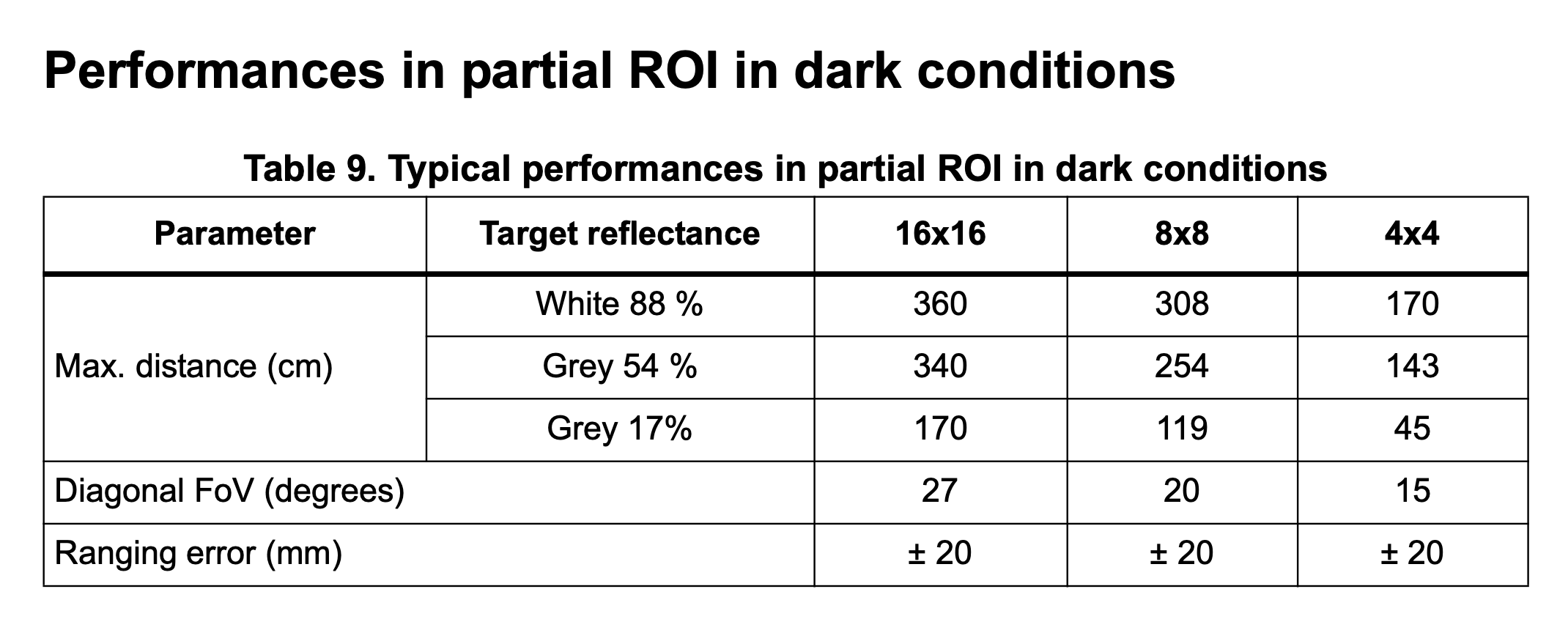
Given the range and angular sensitivity of the TOF sensor as displayed below, I decided to place the two sensors offset from the front middle left and right of the car respectively so that they would have an overlapping field of view (FOV) to provide depth and detect matching information thus providing an error checking mechanism. However, with this configuration the robot will lack "vision" in the surrounding environment outside it's field of view commonly reffered to as a blindspot.

Lab 3(a): Time of Flight Sensors

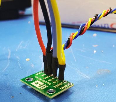
In this segment of the lab, there were a couple things I had to do before communicating with my TOF sensors. First, I connected my two ToF sensors to the Artemis board via soldering. Something uncommon that I had to do during this stage was to daisy chain the connections of my power and I2C lines across my two ToF sensors because of the limited pin connection on the Artemis. See below for what daisy chain setuplooks like.

Next I installed the SparkFun VL53L1X 4m laser distance sensor library from the Arduino IDE. This library enabled me to communicate and configure the ToF to the specifications of my liking. Using one of the library examples, I scanned the I2C channel to find the ToF sensors that I just connected. Upon scanning for one of the sensors, the ToF sensor was found the with I2C address of 0x29 which was a disparity from 0x52 dictated in the datasheet. This happened because the I2C address can be specified two ways: as a base 7-bit address or as an 8-bit address with the LSB a write/read bit. Ideally we'd want to see the address 0x52 however, the problem is that I2C generally refers to the 7-bit address (0x29). So to fix this we'd typically left shift by one to yield to 8bit address (0x52) of the ToF.

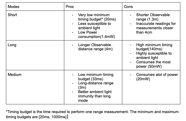
The ToF sensor has three modes that optimize the ranging performance given the maximum expected range. The three modes can be set by the following member function .setDistanceModeShort(), .setDistanceModeMedium(), .setDistanceModeLong(). Depending on the task you want to achieve, each mode has its benefit, but be aware there are tradeoffs to be made for each mode selection. Below is a table of the pros and cons associated with each ranging mode.

Using one of the example codes from the ToF library. I tried to characterize one of the ToF sensors long distance ranging mode abilities. To achieve this, I used a ruler to measure several preset distances and then used the ToF to measure those same distances. In particular I was mostly interested in the ToFs measured range, accuracy, repeatability, and ranging time. See the accompanying graph for the results of this experimennt.

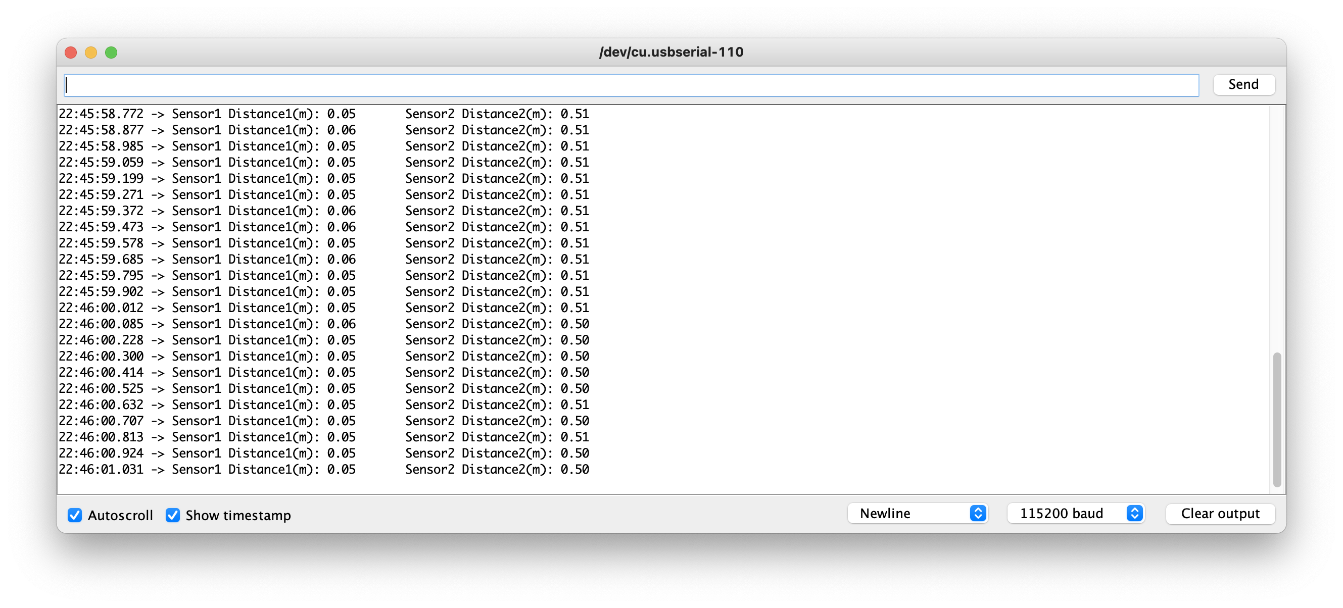
After characterizing the ranging abilities of one of the ToF sensors. I connected the other ToF and ran the same example code (with a few modifications) from the experiment to attempt to read the distances from both sensors simultaneously. Since both ToFs have the same I2C address, I couldn't distinguish which ToF I was communicating with. So to fix this issue, I turned off one of the ToF sensors by driving one of their shutdown pin LOW which allowed me to communicate to the one that was still on. I leveraged this to programmatically change one of the ToF's I2C address and when that was done, I drove the idle ToF's shutdown pin back HIGH and now I could simultaneously read the distance data from both of the ToFs because they now had different addresses. Displayed below is the two ToF sensor's output on the serial monitor.

Lab 3(b): IMU

Accelerometer

In this segment of the lab, I daisy chained the power and I2C lines from the ToF sensors to the IMU. After soldering and establishing the electrical connection between the IMU and the Artemis board, I downloaded the SparkFun 9DOF IMU Breakout Library within the Arduino IDE and ran a basic example program that came with the library. In this example code, I had to modify the value of the parameter called AD0_VAL from 1 to 0. This parameter indicates the value of the last bit of the I2C address of the IMU. On the IMU, there is a jumper that allows you to change the I2C address by a 1-bit difference via hardware. Since this jumper was not connected on the board, the I2C address remained 0x68. However, with a connected jumper the address would have changed to 0x69 and the value of AD0_VAL would remain 1.

The example code basically outputted the values of the accelerometer, gyroscope, and magnetomer to the serial monitor. It printed out the values of acceleration, angular speed, and the magnetic B-field in the X, Y, Z planes. Below are just a few observations I took note of as I moved the sensors in certain directions with certain speeds.

• As I rotated the IMU into X, Y, or Z plane, I noticed the acceleration values of the plane I was currently in would trend towards 1000millig while, the values of the plane I just in / left would trend down towards zero g's.
• With regards to the gyroscope, I also observed that if I rotated the IMU at a constant speed, values of the gyroscope would remain fairly the same. However, if there were any sudden or abprupt movements on the IMU, the gyroscope values would increase drastically compared to its nominal values. I suppose this makes sense as the units of the gyroscope --Degrees per second-- indicate some sort of differential element in the internal calculations.
• Lastly I noticed that whenever I brought my IMU near a magnetic element (my laptop, a charging wire) the values yielded by the magnetometer increased and decreased the farther away the IMU was from the magnetic object.

As mentioned previously, the IMU only outputted values of acceleration, angular speed, magnetic field strength to the serial monitor in the example code. But sometimes, I want know the angle and or orientation on the IMU with all the extra information from the magnetomer, accelerometer, and gyroscope. To make this information more succint, I created two variables--pitch and roll-- that would tell the IMU's angle about the y-axis and x-axis respectively. To retrieve the value of pitch in degrees, I took the arctan of the x-values of the accelerometer divided by the z-values of the accelerometer and multiplied the result by 180/PI. Similarly to retrived the value of roll in degrees, I took the arctan of the y-values of the accelerometer divided by the z-values of the accelerometer and multiplied the result by 180/PI. The readings from the pitch and roll values were pretty accurate as they corresponded to the observable angle of the IMU.

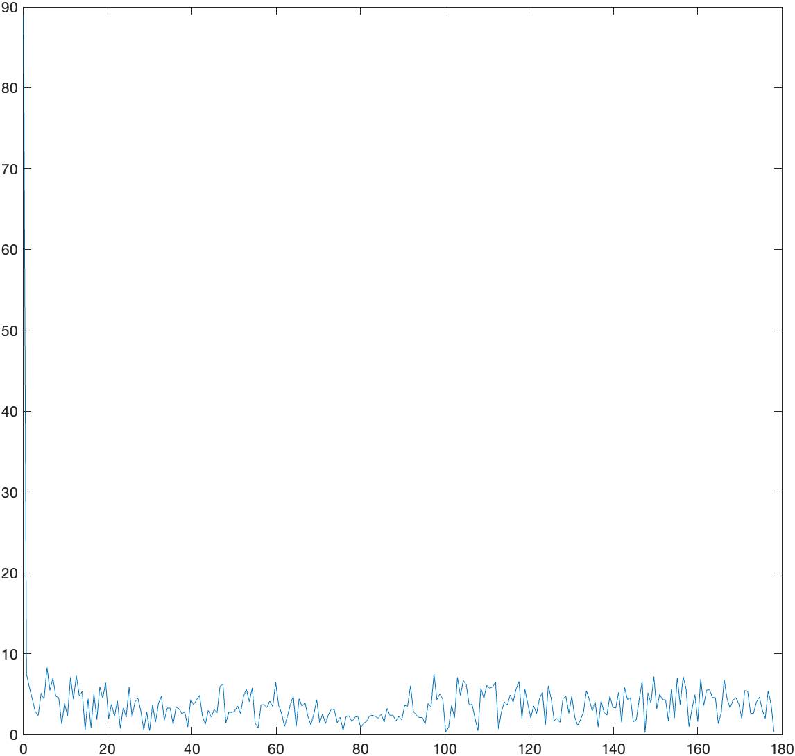
In addition to simplifying the information I was receiveing from the IMU, I also wanted to check how susceptible the IMU device was to noise. If the IMU was heavily susceptible, I would try to mitigate it via a software low-pass filter / averager. Nonetheless, I tested its noise immunity by simply recording the values of the IMU while it was at a stable position and then tapping it a couple times to introduce noise into the system. Next I took the fourier transform of the time domain signal, hoping to find the frequency spectrum of the unwanted noise, so that I can create a complimentary low-pass filter guided by the plot. However, as you can see in the below frequency plot of the data no frequency spikes are evident. Initially I thought I was doing something wrong but it turns out that this plot is actually correct. The reason there are no spikes in magnitude associated with the noise frequency is because the IMU device initial settings has an internal low-pass filter activated which makes it resisilient to the noise coming from the taps. Had the low-pass filter not been turned on, the noise from accelerometer readings would be detectable.

Single-Sided Amplitude Spectrum of Pitch(t)

Gyroscope

Using the gyroscope, I tried to repeat the same task of computing pitch and roll and I noticed a couple properties from the gyroscope. I observed that the gyroscope was far less susceptible to noise and or drastic changes in pitch and roll angles, however, the downside of this attribute is that the gyroscope can accumulate error over time and it might take a while for the gyrosocpe to revert back to the proper measurement values. See below for a plot of the roll data from the gyroscope. Note how the gyroscope's roll values indicate by the orange color takes a while to trend towards the correct value of roll calculated with the accelerometer in red.

Despite the fact that the gyroscope drifts during pitch and roll computations, this issue can be mitigated by increasing the sampling frequency of the IMU sensor. With a higher sampling frequency, we get more data points which allows for a better resolution and ultimately a decrease in drift and an improvement in accuracy.

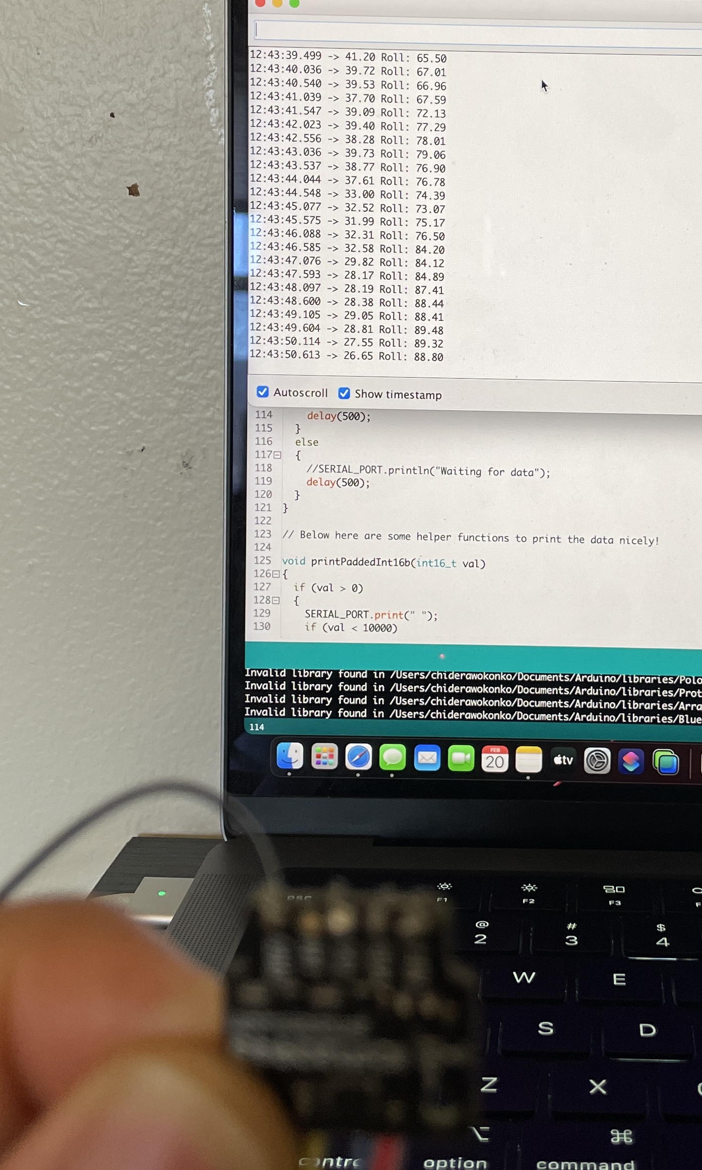
Here you can see that my IMU is vertical, but it takes between 7-8 seconds on the serial monitor for my gyroscope to recalibrate close to my current angle. This is a product of a lower sampling frequency.

Unlike in the previous data set, here you can see that my IMU is also vertical, but it under a second on the serial monitor for my gyroscope to recover my current angle. This is a product of a higher sampling frequency.

So to tie the data from the accelerometer and gyroscope together regarding the pitch and roll angles, I decided to make a complimentary filter that leverages the noise resilience of the gyroscope and the accuracy of the accelerometer. With a simple weighted sum of the two measurement units, I was able produce pitch data that was both accurate and semi-noise immune. See the video below for the complimentary filter plot of the pitch and roll and along side their respective gyroscope and accelerometer readings.

The list below is the legend for the plots featured in the following video

• The Gyroscope data is marked by an orange plot
• The Accelerometer data is marked by a red plot
• The Complimentary filtered data is marked by a black plot

Roll Plot

Note how in both videos the black plot suppresses the noise that appears on the red plot from the accelerometer but also retains the accuracy of the data better than the orange plot of the gyroscope.

Pitch Plot

• GitHub Repository