Awesome Buneary

Exploratory data analysis

Research question(s)

How does coffee’s aroma, flavor, acidity, sweetness, and total score depend on their original country and region?

Data collection and cleaning

Have an initial draft of your data cleaning appendix. Document every step that takes your raw data file(s) and turns it into the analysis-ready data set that you would submit with your final project. Include text narrative describing your data collection (downloading, scraping, surveys, etc) and any additional data curation/cleaning (merging data frames, filtering, transformations of variables, etc). Include code for data curation/cleaning, but not collection.

library(tidyverse)

── Attaching packages ─────────────────────────────────────── tidyverse 1.3.2 ──
✔ ggplot2 3.4.2     ✔ purrr   1.0.0
✔ tibble  3.2.1     ✔ dplyr   1.1.2
✔ tidyr   1.2.1     ✔ stringr 1.5.0
✔ readr   2.1.3     ✔ forcats 0.5.2
── Conflicts ────────────────────────────────────────── tidyverse_conflicts() ──
✖ dplyr::filter() masks stats::filter()
✖ dplyr::lag()    masks stats::lag()

library(tidymodels)

── Attaching packages ────────────────────────────────────── tidymodels 1.0.0 ──
✔ broom        1.0.2     ✔ rsample      1.1.1
✔ dials        1.1.0     ✔ tune         1.1.1
✔ infer        1.0.4     ✔ workflows    1.1.2
✔ modeldata    1.0.1     ✔ workflowsets 1.0.0
✔ parsnip      1.0.3     ✔ yardstick    1.1.0
✔ recipes      1.0.6     
── Conflicts ───────────────────────────────────────── tidymodels_conflicts() ──
✖ scales::discard() masks purrr::discard()
✖ dplyr::filter()   masks stats::filter()
✖ recipes::fixed()  masks stringr::fixed()
✖ dplyr::lag()      masks stats::lag()
✖ yardstick::spec() masks readr::spec()
✖ recipes::step()   masks stats::step()
• Learn how to get started at https://www.tidymodels.org/start/

library(openintro)

Loading required package: airports
Loading required package: cherryblossom
Loading required package: usdata

Attaching package: 'openintro'

The following object is masked from 'package:modeldata':

    ames

library(skimr)
library(scales)
coffee <- read.csv("data/coffee.csv")
coffee <- coffee |>
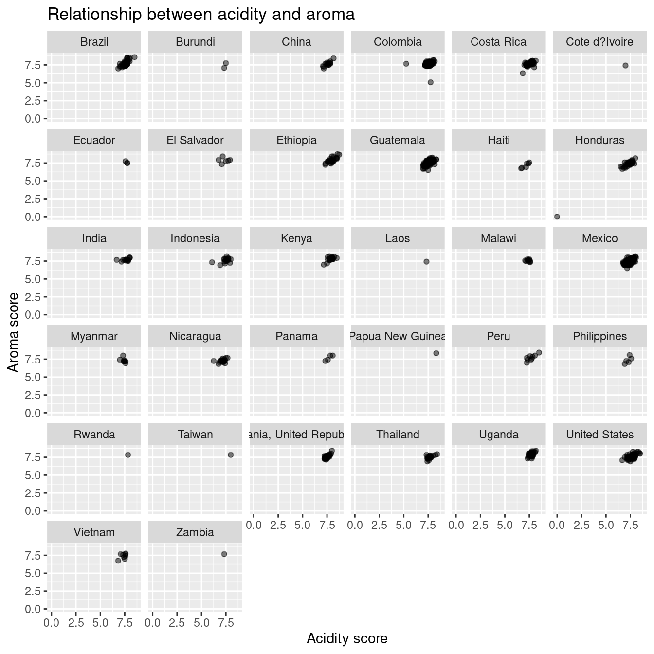
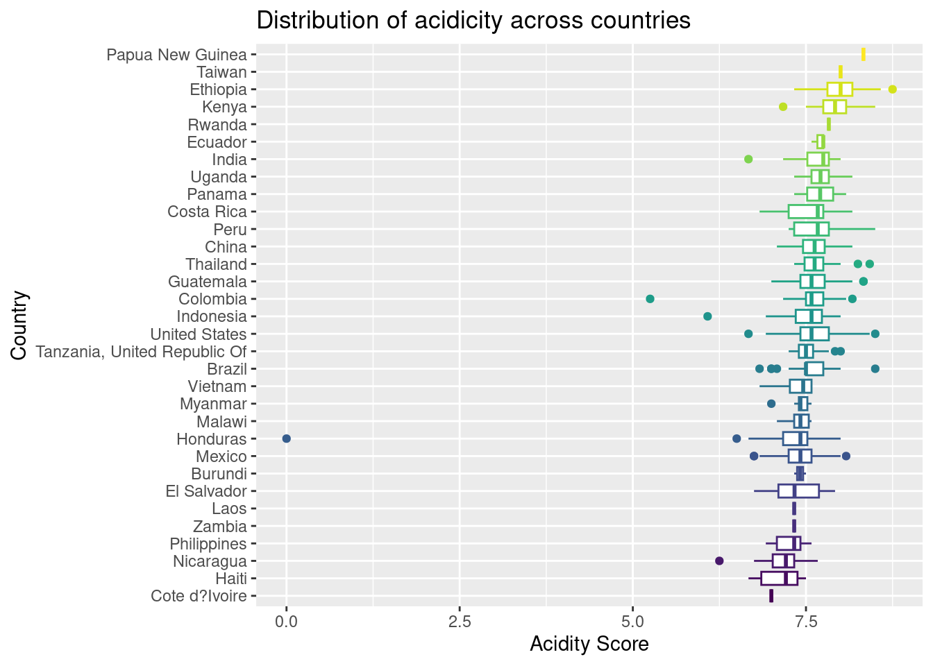
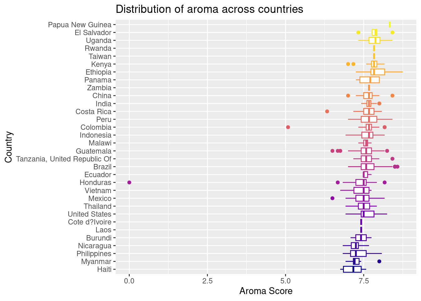
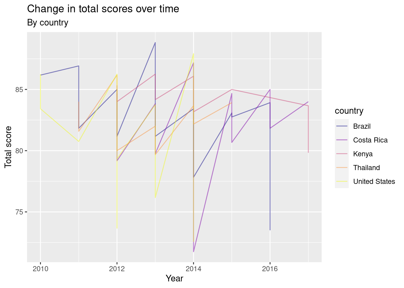
  select(Location.Country, Location.Region, Year, Data.Type.Species, Data.Scores.Aroma, Data.Scores.Flavor, Data.Scores.Aftertaste, Data.Scores.Acidity, Data.Scores.Balance, Data.Scores.Sweetness, Data.Scores.Moisture, Data.Scores.Total) |>
  rename(country = Location.Country, region = Location.Region, year = Year, species = Data.Type.Species, aroma_score = Data.Scores.Aroma, flavor_score = Data.Scores.Flavor, aftertaste_score = Data.Scores.Aftertaste, acidity_score = Data.Scores.Acidity, balance_score = Data.Scores.Balance, sweetness_score = Data.Scores.Sweetness, moisture_score = Data.Scores.Moisture, total_score = Data.Scores.Total)

Data Collection

The coffee dataset was downloaded from a public repository, which was obtained by downloading a CSV file from https://think.cs.vt.edu/corgis/csv/coffee/. It contains information on the country and region where the coffee was produced, the year of production, the type of coffee species, and scores for various attributes such as aroma, flavor, acidity, balance, sweetness, and moisture. The purpose of our analysis was to examine the relationship between the scores for each of these attributes and their original country and region.

Data Cleaning Steps

We first created a dataset called coffee using the csv file we downloaded.
We select the columns that we need for our research questions, and we also selected some columns that are not in our question, but we think we might use.
We rename the columns to names that are easy to use and identify.
We used the is.na() function to check for missing values in the dataset. Fortunately, there were no missing values in the dataset, so we did not need to impute any values.
We used the duplicated() function to check for duplicate rows in the dataset. We found that there were no duplicate rows.
We used the skim() function from the skimr package to generate summary statistics for each column in the dataset, including minimum and maximum values, mean, standard deviation, and percentiles. We used this information to identify potential outliers in the data.

Data description

The team found the data set on https://think.cs.vt.edu/corgis/csv/coffee/, which is a data project by Austin Cory Bart, Dennis Kafura, Clifford A. Shaffer, Javier Tibau, Luke Gusukuma, and Eli Tilevich, according to the website. This project was created by Professor Luther Tychonievich of the University of Virginia, and was initially funded by a National Science Foundation grant awarded to Tychonievich in 2014. The project later received additional funding from the University of Virginia and the Mozilla Foundation. The project was created to solve the lack of high-quality, real-world datasets that are interesting and engaging for students and instructors to work with. The data sets are usually easily to look at, visualize, and analyze. The selected data set is “coffee.” According to the website, this data comes from Buzzfeed Data Scientist James LeDoux, and were collected from “the Coffee Quality Institute’s review pages in January 2018.” The reason of the creation of this data set is unspecified on the website, but based on the team’s speculation, it might be used for coffee analysis for professionals or for coffee business researchers. Based on the goal of the CORGIS project, this data set might also be used for students and instructors for data analysis. The data set consists of categorical and numerical data. The data set contains attributes for Arabica and Robusta beans (categorical), from many countries and regions (categorical) and rated on a 0-100 scale (numerical) for categories such as acidity, sweetness, fragrance, balance, etc. Each observation contains the specific data of one type of coffee, and the attributes including bean type, countries, regions, acidity, sweetness, fragrance, balance… The fact that the data was collected from a coffee quality review might have influenced the data collected, as the review would focus more on the quality, type, and country, rather than other factors, such as price. The earliest data was in 2010, which might be the earliest year in which the review was initiated. The team pre-processed the data by renaming the attributes (column names) into more explicit and self-explanatory ones. For example, country replaces Location.Country, region replaces Location.Region, aroma_score replaces Data.Scores.Aroma. The team did not make additional changes to the data set at this stage since it is already well-organized. This data set solely consists of data of coffee and does not involve any data on people, hence we do not expect to encounter ethical issues while working on the data.

Data limitations

Identify any potential problems with your dataset.

The dataset is not very recent, as it was published in 2010, which means in the past 13 years, the locations of grown coffee might have slightly changed or been added, or maybe new strains of Arabica and Robusta coffee beans might have been introduced since then. Therefore, analyzing this data in the hopes of understanding the most recent trends and spreads of coffee quality and characteristics around the world might not lead to the most accurate result.

In addition, the scales that measure certain qualities of coffee seem to be limited. Even though there is a coffee cupping procedure that is designed to measure and distinguish the difference between the flavor and bitterness of coffee from different regions numerically, it can be debated that this type of measurement is a qualitative measurement that is trying to be made quantitative in order to fit the dataset needs. Therefore, this data is limited in its credibility if it is looked at it from this view. However, this limitation is questionable because the scores are verified by the professional method of cuppers. Therefore, this problem is only applicable if people do not approve of the credibility of the cupping method used to create this dataset, and believe that the scores for coffee beans from certain regions are biased because of this.

Exploratory data analysis

Perform an (initial) exploratory data analysis.

#possible research question: How does coffee's aroma, flavor, acidity, sweetness, and total score depend on their original country and region?

glimpse(coffee)

Rows: 989
Columns: 12
$ country          <chr> "United States", "Brazil", "Brazil", "Ethiopia", "Eth…
$ region           <chr> "kona", "sul de minas - carmo de minas", "sul de mina…
$ year             <int> 2010, 2010, 2010, 2010, 2010, 2010, 2010, 2010, 2010,…
$ species          <chr> "Arabica", "Arabica", "Arabica", "Arabica", "Arabica"…
$ aroma_score      <dbl> 8.25, 8.17, 8.42, 7.67, 7.58, 7.50, 7.67, 7.25, 7.42,…
$ flavor_score     <dbl> 8.42, 7.92, 7.92, 8.00, 7.83, 7.92, 7.58, 7.25, 7.42,…
$ aftertaste_score <dbl> 8.08, 7.92, 8.00, 7.83, 7.58, 7.42, 7.50, 7.25, 7.50,…
$ acidity_score    <dbl> 7.75, 7.75, 7.75, 8.00, 8.00, 7.67, 7.58, 7.33, 7.92,…
$ balance_score    <dbl> 7.83, 8.00, 8.00, 7.83, 7.50, 7.58, 7.58, 8.00, 7.58,…
$ sweetness_score  <dbl> 10.00, 10.00, 10.00, 10.00, 10.00, 10.00, 10.00, 10.0…
$ moisture_score   <dbl> 0.00, 0.08, 0.01, 0.00, 0.10, 0.01, 0.00, 0.10, 0.05,…
$ total_score      <dbl> 86.25, 86.17, 86.17, 85.08, 83.83, 83.42, 83.08, 80.3…

#mean aroma, flavor, sweetness by country 
coffee |> 
  group_by(country) |> 
  summarize(mean(aroma_score), mean(acidity_score),
            mean(flavor_score), mean(sweetness_score), mean(total_score))

# A tibble: 32 × 6
   country       `mean(aroma_score)` `mean(acidity_score)` `mean(flavor_score)`
   <chr>                       <dbl>                 <dbl>                <dbl>
 1 Brazil                       7.68                  7.55                 7.64
 2 Burundi                      7.42                  7.42                 7.46
 3 China                        7.64                  7.58                 7.63
 4 Colombia                     7.67                  7.59                 7.61
 5 Costa Rica                   7.65                  7.55                 7.51
 6 Cote d?Ivoire                7.42                  7                    7.25
 7 Ecuador                      7.58                  7.69                 7.64
 8 El Salvador                  7.86                  7.36                 7.79
 9 Ethiopia                     7.92                  8.02                 8.01
10 Guatemala                    7.55                  7.60                 7.49
# ℹ 22 more rows
# ℹ 2 more variables: `mean(sweetness_score)` <dbl>, `mean(total_score)` <dbl>

# mean aroma, flavor, sweetness by region 
coffee |> 
  group_by(region) |>
  summarize(mean(aroma_score),  mean(acidity_score),
            mean(flavor_score), mean(sweetness_score), mean(total_score))

# A tibble: 278 × 6
   region         `mean(aroma_score)` `mean(acidity_score)` `mean(flavor_score)`
   <chr>                        <dbl>                 <dbl>                <dbl>
 1 acatenango                    7.75                  8.06                 7.89
 2 aceh                          7.83                  7.33                 7.58
 3 aceh gayo                     7.5                   7.42                 7.5 
 4 aceh tengah                   7.81                  7.75                 7.88
 5 addis ababa                   7.83                  8.17                 8   
 6 adolfo lopez …                7.58                  7.67                 7.67
 7 aldea xeucalv…                7.58                  8                    7.75
 8 alta paulista…                7.58                  7.25                 7.42
 9 altotonga                     7.5                   7.5                  7.58
10 amatenango de…                7.58                  7.42                 7.42
# ℹ 268 more rows
# ℹ 2 more variables: `mean(sweetness_score)` <dbl>, `mean(total_score)` <dbl>

# number of countries per region 
coffee |> 
  group_by(region) |> 
  count(country)

# A tibble: 298 × 3
# Groups:   region [278]
   region                                           country       n
   <chr>                                            <chr>     <int>
 1 acatenango                                       Guatemala     3
 2 aceh                                             Indonesia     1
 3 aceh gayo                                        Indonesia     1
 4 aceh tengah                                      Indonesia     1
 5 addis ababa                                      Ethiopia      1
 6 adolfo lopez mateos                              Mexico        1
 7 aldea xeucalvitz, ixil region, quiche department Guatemala     1
 8 alta paulista (sao paulo)                        Brazil        1
 9 altotonga                                        Mexico        1
10 amatenango de la frontera                        Mexico        1
# ℹ 288 more rows

ggplot(coffee, aes(x = acidity_score, y = aroma_score)) + 
  geom_point(alpha = 0.5) + 
  facet_wrap(vars(country)) + 
  labs( 
    x = "Acidity score",
    y = "Aroma score",
    title = "Relationship between acidity and aroma",
    subtile = "By country"
      )

coffee |> 
  mutate(
    country = parse_factor(x = country),
    country = fct_reorder(
      .f = country,
      .x = acidity_score
      )
    ) |>
  ggplot(aes(y = country, x = acidity_score, color = country)) + 
  geom_boxplot(show.legend = FALSE) + 
  scale_color_viridis_d(option = "D") + 
  labs(
    x = "Acidity Score",
    y = "Country",
    title = "Distribution of acidicity across countries"
  )

coffee |> 
  mutate(
    country = parse_factor(x = country),
    country = fct_reorder(
      .f = country,
      .x = aroma_score
      )
    ) |>
  ggplot(aes(y = country, x = aroma_score, color = country)) + 
  geom_boxplot(show.legend = FALSE) + 
  scale_color_viridis_d(option = "C") + 
  labs(
    x = "Aroma Score",
    y = "Country",
    title = "Distribution of aroma across countries"
  )

# selected countries in different continental regions 
# North America, Asia, South America, Africa, and Central America 
countries_of_interest <- c("United States", "Thailand", "Brazil", 
                           "Kenya", "Costa Rica")
coffee |> 
  filter(country %in% countries_of_interest) |> 
  ggplot(aes(x = year, y = total_score, color = country)) + 
  geom_line(alpha = 0.5) + 
  scale_color_viridis_d(option = "C") + 
  labs(
    x = "Year",
    y = "Total score",
    title = "Change in total scores over time", 
    subtitle = "By country"
  )

Questions for reviewers

List specific questions for your peer reviewers and project mentor to answer in giving you feedback on this phase.

Should we considering combining with another dataset to make our question more nuanced? (We have a dataset on state fragility that could be used to see if coffee production is correlated with it)
Are there any specific comparisons of coffee qualities vs. locations that we should analyze or emphasize?