An Analysis of NYPD Arrest Data
Report
Introduction
For our research project we decided to analyze the 2022 arrest data for NYC and see if we could find some noticeable trends or patterns. Our motivation for choosing the dataset was to see the effectiveness of law enforcement and assessing racial and socioeconomic disparities to understand if there were biases. Some questions we asked were:
Is there a relationship between crime perpetrator characteristics and the level of offense they are charged with?
Is there is a relationship between borough and crime perpetrator characteristics?
Are there noticeable trends in when arrests are made throughout the year/month?
For the first question, we found that perpetrators tend to be men and black people are the most likely to be arrested and convicted of higher level offenses. For the second, we specifically analyzed female arrests in Staten Island vs. the other boroughs and found that the proportion in Staten Island to be statistically significantly different. Finally, we also noticed trends where throughout the month the number of arrests decreased and that the winter months (December, January, and February) had the lowest arrests compared to the other months. However there was no statistically significant observed difference in the timing of arrests in the month and the characteristics of the perpetrators.
Data description
This data set was created to track all NYC arrests in a public database. It allows the police department to keep track of crimes as well as keep the public informed on their operations. It was extracted by the Office of Management Analysis and Planning and has been organized from crime reports. The data could have been influenced by police perceptions at the moment of the crime (potential biases) as police had to fill out all the details for each crime report they created. There might also lost cases due to human error as a result of the manual data extraction. The police probably know the data is being collected and stored somewhere but the people being arrested probably don’t. The lack of awareness the perpetrator may have for the data being collected and where it is going creates some ethical concern as people may be able to identify candidates in the dataset given the characteristics. While names are not included, the date, race, sex, age, and more of the perpetrator are and a google search of crimes on that date in NYC could reveal the identity of the perpetrator. The police probably expect the data to be used for public awareness given how public information is becoming nowadays.
To prepare the data for this report we had to due some cleaning steps. This included selecting necessary columns while dropping unnecessary ones, completing variable names to make them more legible, and reordering and condensing factor levels to make the visualizations more concise. Exact changes made to the data for each analysis are described below at corresponding sections of the report.
Each row is a individual arrest.
Each column represents a different tracked variable. We chose to keep 12 of them. These 12 are:
ARREST_KEY = Randomly generated persistent ID for each arrest
ARREST_DATE = Exact date of arrest for the reported event
PD_CD = Three digit internal classification code (more granular than Key Code)
PD_DESC = Description of internal classification corresponding with PD code (more granular than Offense Description)
KY_CD = Three digit internal classification code (more general category than PD code)
OFNS_DESC = Description of internal classification corresponding with KY code (more general category than PD description)
LAW_CODE = Law code charges corresponding to the NYS Penal Law, VTL and other various local laws
LAW_CAT_CD = Level of offense: felony, misdemeanor, violation
ARREST_BORO = Borough of arrest. B(Bronx), S(Staten Island), K(Brooklyn), M(Manhattan), Q(Queens)
AGE_GROUP = Perpetrator’s age within a category
PERP_SEX = Perpetrator’s sex description
PERP_RACE = Perpetrator’s race description
Data analysis
# A tibble: 187,457 × 12
   ARREST_KEY ARREST_DATE PD_CD PD_DESC      KY_CD OFNS_DESC LAW_CODE LAW_CAT_CD
        <dbl> <chr>       <dbl> <chr>        <dbl> <chr>     <chr>    <chr>
 1  239553009 01/23/2022    464 JOSTLING       230 JOSTLING  PL 1652… M
 2  239922214 01/31/2022    397 ROBBERY,OPE…   105 ROBBERY   PL 1601… F
 3  239939130 02/01/2022    105 STRANGULATI…   106 FELONY A… PL 1211… F
 4  240521791 02/13/2022    101 ASSAULT 3      344 ASSAULT … PL 1200… M
 5  241022365 02/21/2022    397 ROBBERY,OPE…   105 ROBBERY   PL 1600… F
 6  242064428 03/14/2022    105 STRANGULATI…   106 FELONY A… PL 1211… F
 7  242456937 03/22/2022    105 STRANGULATI…   106 FELONY A… PL 1211… F
 8  242818613 03/29/2022    705 FORGERY,ETC…   358 OFFENSES… PL 1702… M
 9  243132247 04/05/2022    157 RAPE 1         104 RAPE      PL 1303… F
10  244567670 05/04/2022    109 ASSAULT 2,1…   106 FELONY A… PL 1200… F
# ℹ 187,447 more rows
# ℹ 4 more variables: ARREST_BORO <chr>, AGE_GROUP <chr>, PERP_SEX <chr>,
#   PERP_RACE <chr>
Analysis #1
Is there a relationship between crime perpetrator characteristics and the level of offense they are charged with. Is there a potential for people of different races/sexes/ages being charged different levels of offense for a crime that falls under the same law code?
For analysis 1 we decided to collapse the LAW_CAT_CD variable in to just 3 factors instead of 4 as infractions and violations were essentially the same level and appeared very infrequently in the dataset. Thus we ended with 3 levels for LAW_CAT_CD violation, misdemeanor, and felony.
# A tibble: 6 × 5
  term                            estimate std.error statistic p.value
  <chr>                              <dbl>     <dbl>     <dbl>   <dbl>
1 (Intercept)                       13346.       NaN       NaN     NaN
2 PERP_SEXM                         58296        NaN       NaN     NaN
3 LAW_CAT_CDViolation              -13226.       NaN       NaN     NaN
4 LAW_CAT_CDMisdemeanor              6134.       NaN       NaN     NaN
5 PERP_SEXM:LAW_CAT_CDViolation    -57502.       NaN       NaN     NaN
6 PERP_SEXM:LAW_CAT_CDMisdemeanor    4179.       NaN       NaN     NaN
# A tibble: 6 × 4
# Groups: PERP_SEX, LAW_CAT_CD [6]
PERP_SEX LAW_CAT_CD ARRESTS PERCENT
<chr> <fct> <int> <dbl>
1 F Felony 13346 0.0712
2 F Misdemeanor 19480 0.104
3 F Violation 120 0.000640
4 M Felony 71642 0.382
5 M Misdemeanor 81955 0.437
6 M Violation 914 0.00488 # A tibble: 7 × 3
# Groups: PERP_RACE [7]
PERP_RACE ARRESTS PERCENT
<chr> <int> <dbl>
1 AMERICAN INDIAN 516 0.00275
2 ASIAN 10085 0.0538
3 BLACK 93229 0.497
4 BLACK HISPANIC 17139 0.0914
5 UNKNOWN 673 0.00359
6 WHITE 19158 0.102
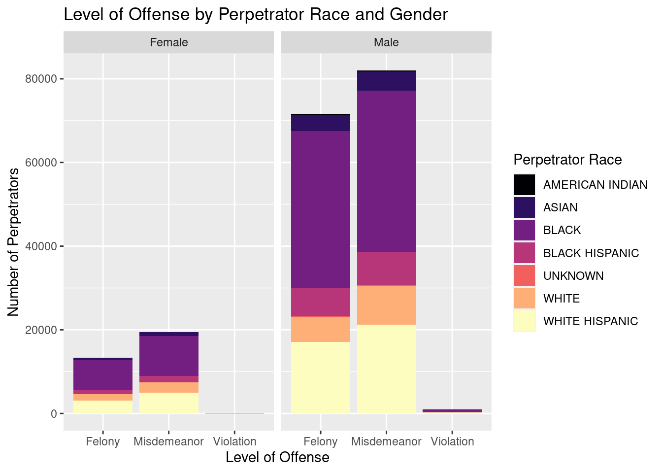
7 WHITE HISPANIC 46657 0.249 Below is a formula modelling the expected number of arrests in a year given a perpetrators gender and level of offense. An interpretation of it would be that for a female perpetrator with a felony we would expect on average 13346 arrests. For women with misdemeanors we would expect on average 6134 more arrests. For women with violations we would expect on average 13226 less arrests. For a male perpetrator with a felony we would expect on average 58296 more arrests. For men with misdemeanors we would expect on average 4179 more arrests. For men with violations we would expect on average 57502 less arrests.
\[ \begin{split} \widehat{ARRESTS} = 13346 + MALE \times 58296 + Violation \times -13226 + Misdemeanor \times 6134 + \\ MALE \times Violation \times -57502 + MALE \times Misdemeanor \times 4179 \end{split} \]
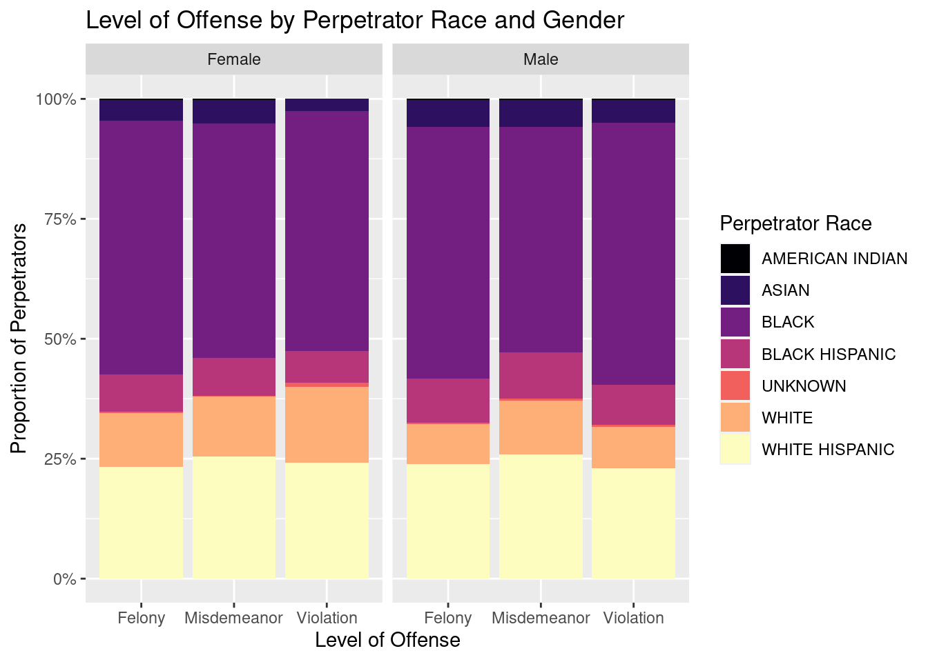
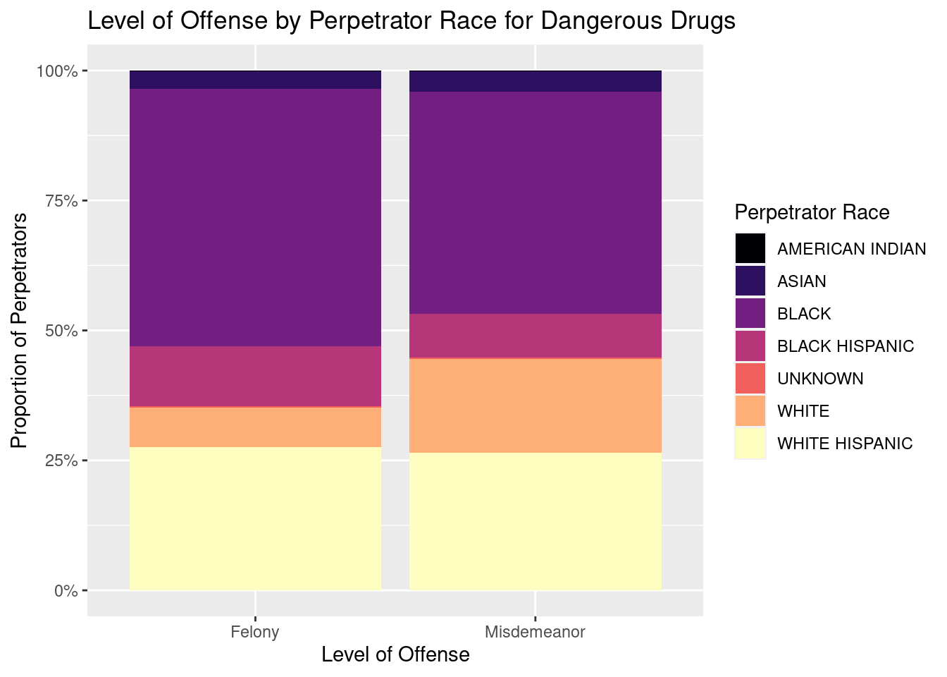
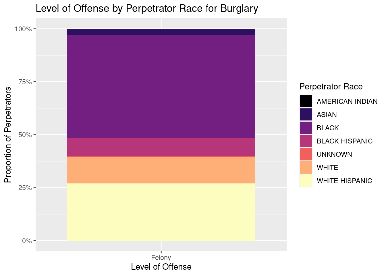
Looking at the bar graphs for “Level of Offense by Perpetrator Race and Gender there are some common trends that appear. First, a majority of the crimes in this data set are misdemeanors followed by felonies with only a few being violations. Second, perpetrators tend to be men with more than 4x more men than women being charged for misdemeanors and nearly 5.5x more men being charged for felonies than women. Another interesting data point is that black people are the most likely to be arrested with nearly 4.5x more black people than white people appearing in this dataset. The race that appeared the least in this dataset is american indians with just over 500 people compared to the 19000 white people and 93000 black people. Another interesting component is that white hispanics are nearly 3x as likely to be in arrested than black hispanics. Finally, looking at a few graphs of level of offense by perpetrator race and the offense code assigned to the arrest revealed a couple interesting things. First, it appears that for a lot of the codes, there is uniform assignment of level of offense. For instance, all 3rd degree assaults were charged as misdemeanors and all burglaries were felonies. An exception to this rule is the”dangerous drugs” offense code which sees some arrests assigned to misdemeanors and others to felonies. Interestingly, black people made up a larger proportion of the “dangerous drugs” offenses that were charged as felonies than misdemeanors and white people made up a larger proportion of offenses that were charged as misdemeanors than felonies.
Analysis #2
Our second research question is there a relationship between borough and crime perpetrator characteristics. Do certain boroughs have higher percentages of men or women committing crimes?
# A tibble: 2 × 2
  PERP_SEX   pct
  <chr>    <dbl>
1 F        0.176
2 M        0.824
# A tibble: 10 × 3
# Groups: ARREST_BORO [5]
ARREST_BORO PERP_SEX pct
<chr> <chr> <dbl>
1 B F 0.188
2 B M 0.812
3 K F 0.170
4 K M 0.830
5 M F 0.165
6 M M 0.835
7 Q F 0.177
8 Q M 0.823
9 S F 0.197
10 S M 0.803From the two tables, there doesn’t appear to be a large difference in perpetrator by sex. Since Staten Island has the greatest difference from the citywide average, I will compare the two to see if the difference is significant.
Analysis #3
Are there trends between time of year and number of arrests made? Do these trends look different across different misdemeanors, races, boroughs, ages, or genders?
For our third analysis we separated the date column from one date in to month, day, and year columns for each date to make analysis of the time series data easier.
# A tibble: 187,457 × 9
   ARREST_KEY MONTH   DAY  YEAR OFNS_DESC           AGE_GROUP PERP_SEX PERP_RACE
        <dbl> <fct> <int> <int> <chr>               <chr>     <chr>    <chr>
 1  239553009 Jan      23  2022 JOSTLING            25-44     M        BLACK
 2  239922214 Jan      31  2022 ROBBERY             25-44     M        BLACK
 3  239939130 Feb       1  2022 FELONY ASSAULT      65+       M        WHITE
 4  240521791 Feb      13  2022 ASSAULT 3 & RELATE… 45-64     M        BLACK
 5  241022365 Feb      21  2022 ROBBERY             45-64     M        BLACK
 6  242064428 Mar      14  2022 FELONY ASSAULT      <18       M        BLACK
 7  242456937 Mar      22  2022 FELONY ASSAULT      18-24     M        BLACK
 8  242818613 Mar      29  2022 OFFENSES INVOLVING… 25-44     M        BLACK
 9  243132247 Apr       5  2022 RAPE                45-64     M        BLACK HI…
10  244567670 May       4  2022 FELONY ASSAULT      25-44     F        BLACK
# ℹ 187,447 more rows
# ℹ 1 more variable: ARREST_BORO <chr>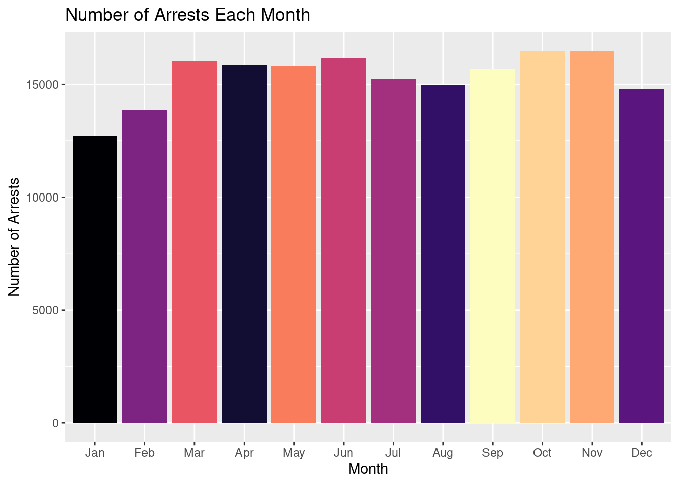
# A tibble: 12 × 2
   MONTH ARRESTS
   <fct>   <int>
 1 Jan     13037
 2 Apr     15885
 3 Aug     15547
 4 Dec     15164
 5 Feb     13895
 6 Jul     15575
 7 Jun     16175
 8 Mar     16712
 9 May     16378
10 Nov     16477
11 Oct     16920
12 Sep     15692
Looking at this tibble we can see the total number of arrests made for each month. The mean number of arrests in a month is 15354.42 and the standard deviation of 1127.69.
To visualize and model the relationship between day of the month and number of arrests we had to make a few transformations. First, we filtered to only include days from 1 to 30 as the number 31 only appears in a few months. This would likely skew the model to have a stronger negative correlation as there would be less total arrests made on the day 31. We also divided the totals for the other 30 days by 12 to get an average number of arrests made for that day of the month.
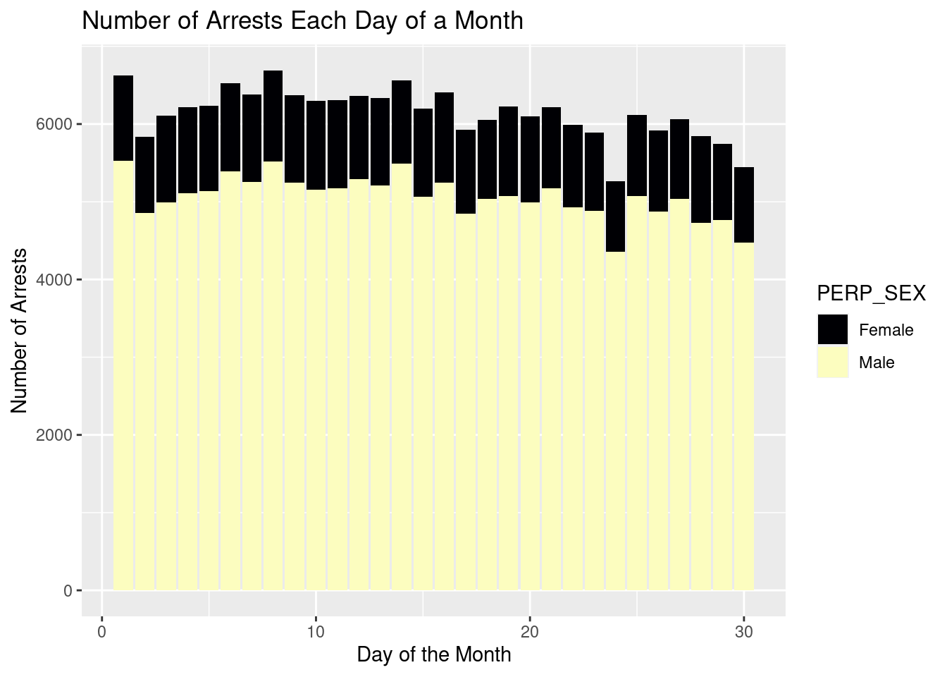
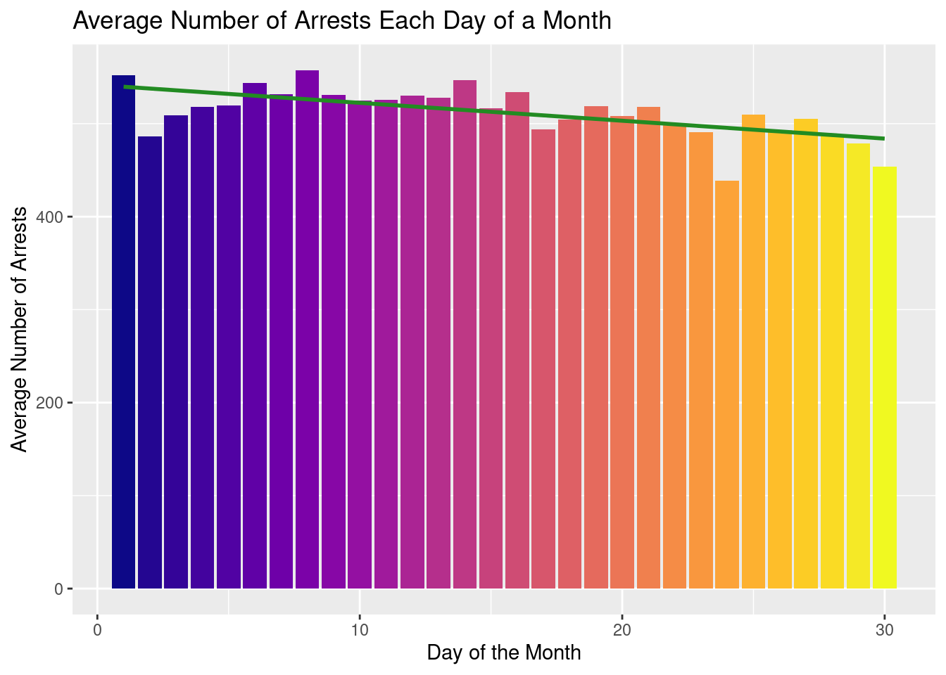
Below is a formula created to model the average number of arrests made on a given day in the month. An interpretation of this model would be that on the first day of the month we would expect an average of 541.63 arrests to be made and that each subsequent day of the month the average number of arrests would decrease by 1.92 arrests.
# A tibble: 2 × 5
  term        estimate std.error statistic  p.value
  <chr>          <dbl>     <dbl>     <dbl>    <dbl>
1 (Intercept)   542.       7.91      68.4  1.02e-32
2 DAY            -1.92     0.446     -4.32 1.80e- 4
\[ \begin{split} \widehat{ARRESTS} = 541.63 + DAY \times -1.92 \end{split} \]
Below is a formula created to model the average day an arrest occurs during the month depending on the perpetrator sex. An interpretation for this model would be that on average arrests of female perpetrators are made on the 15.24 day of the month and the day of the month would decrease one average by 0.03 for male perpetrators.
# A tibble: 2 × 5
  term        estimate std.error statistic p.value
  <chr>          <dbl>     <dbl>     <dbl>   <dbl>
1 (Intercept)  15.2       0.0477   319.      0
2 PERP_SEXM    -0.0303    0.0525    -0.577   0.564
\[ \begin{split} \widehat{DAY} = 15.24 + MALE \times -0.03 \end{split} \]
Evaluation of significance
Evaluation of Significance #1
Null hypothesis race: The true proportion of black perpetrators arrested for felonies is the same white perpetrators
\[H_0: p_b = p_w\]
Alternative hypothesis race: The true proportion of black perpetrators arrested for felonies is not the the same as white perpetrators
\[H_A: p_b \neq p_w\]
For this analysis we had to filter for perpetrators who’s race was white or black.
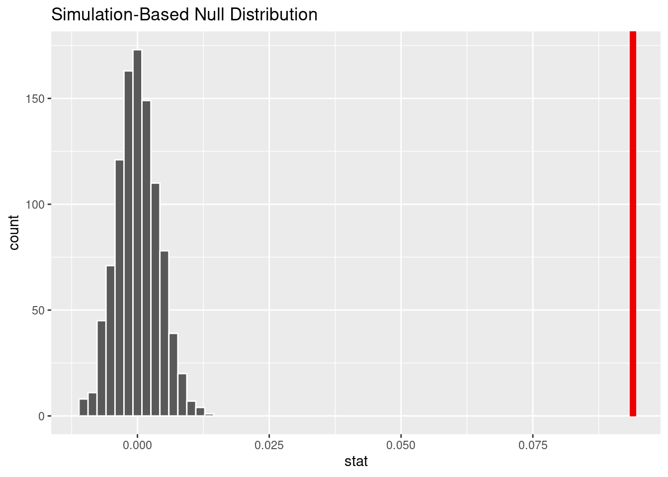
The point estimate, 0.094 represents the observed difference in proportion of felonies for black vs white perpetrators.
We generated the null distribution of difference in proportion of felonies for black vs white perpetrators through permutation 1000 times.
# A tibble: 1 × 1
  p_value
    <dbl>
1       0
Due to the p-value less than 0.05, we reject the null hypothesis. There is significant evidence that the true proportion of black perpetrators arrested for felonies is different than the true proportion of white perpetrators arrested for felonies.
------------------------------------------------------------------------------------------
Null hypothesis sex: The true proportion of male perpetrators arrested for felonies is the same as female perpetrators
\[H_0: p_m = p_f\]
Alternative hypothesis sex: The true proportion of male perpetrators arrested for felonies is not the same as female perpetrators
\[H_A: p_m \neq p_f\]
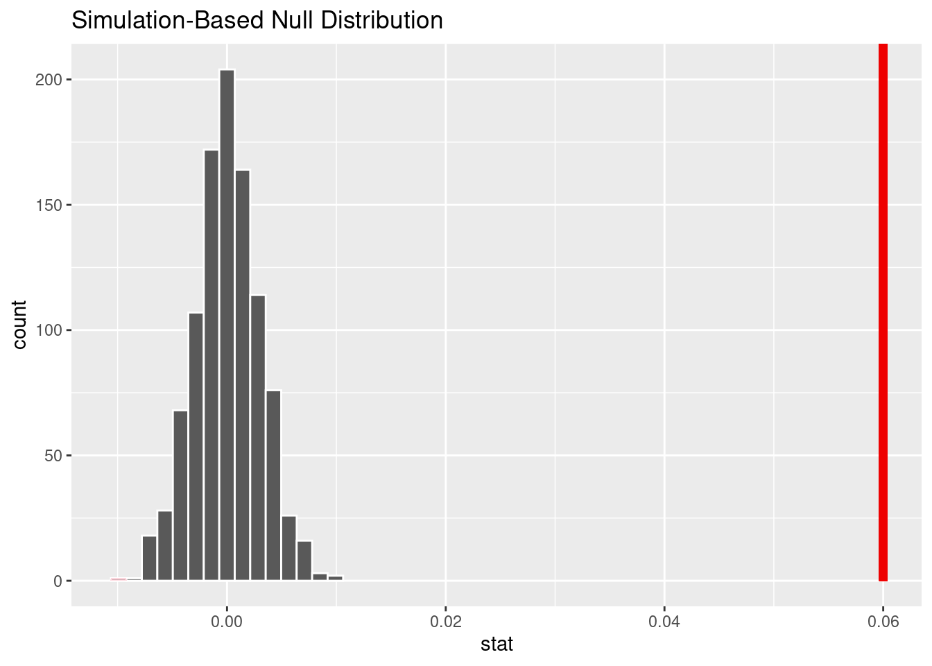
The point estimate, 0.06 represents the observed difference in proportion in felonies for male vs female perpetrators.
We generated the null distribution of difference in proportion of felonies for male vs female perpetrators through permutation 1000 times.
# A tibble: 1 × 1
  p_value
    <dbl>
1       0
Due to the p-value less than 0.05, we reject the null hypothesis. There is significant evidence that the true proportion of men arrested for felonies is different than the true proportion of women arrested for felonies.
------------------------------------------------------------------------------------------
Null hypothesis offense: The true proportion of black perpetrators arrested for dangerous drugs who were convicted of felonies is the same as white perpetrators
\[H_0: p_b = p_w\]
Alternative hypothesis offense: The true proportion of black perpetrators arrested for dangerous drugs who were convicted of felonies is the same as white perpetrators
\[H_A: p_b \neq p_w\]
For this analysis we had to filter for only white and black perpetrators who’s offense description was ‘dangerous drugs’.
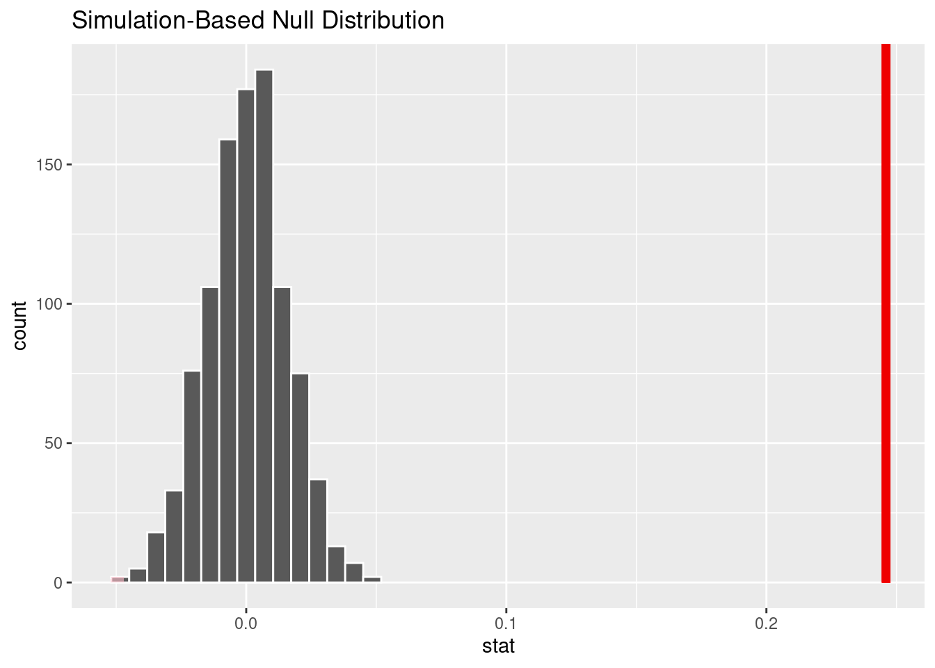
The point estimate, 0.246 represents the observed difference in proportion of felonies for black vs white perpetrators arrested for for dangerous drugs.
We generated the null distribution of difference in proportion of felonies for black vs white perpetrators for ‘dangerous drugs’ arrests through permutation 1000 times.
# A tibble: 1 × 1
  p_value
    <dbl>
1       0
With a p-value less than 0.05, we reject the null hypothesis. There is significant evidence that the true proportion of black perpetrators arrested for dangerous drugs who were convicted of felonies is not the same as white perpetrators
Evaluation of Significance #2
Based on the initial analysis, the hypothesis we test is as follows:
Null hypothesis: The true proportion of female perpetrators in Staten Island is the same as citywide
\[H_0: p_c = p_s\]
Alternative hypothesis: The true proportion of female perpetrators in Staten Island is not the same as citywide
\[H_A: p_c \neq p_s\]
For this analysis, we have to classify the boroughs as either Staten Island or not.
We can then calculate the point estimate, which tells us what the observed proportion of female perpetrators in Staten Island was: 0.023.
We generated the null distribution of difference in proportion of arrests of female perpetrators on Staten Island vs the rest of the city through permutation 1000 times.
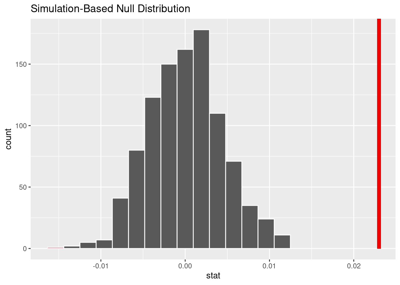
This is the visualization of that null distribution and the p-value.
# A tibble: 1 × 1
  p_value
    <dbl>
1       0
Due to the p-value less than 0.05, we reject the null hypothesis. There is significant evidence that the true proportion of females perpetrators in Staten Island is different than the true proportion of females perpetrators in other boroughs.
Evaluation of Significance #3
If the correlation between day and number of arrests is significant, the hypothesis would be as follows:
Null hypothesis: There is no correlation between day of the month and number of arrests
\[H_0: \beta = 0\]
Alternative hypothesis: There is a correlation between day of the month and number of arrests
\[H_A: \beta \neq 0\]
The fit of the model is as follows:
# A tibble: 2 × 5
  term        estimate std.error statistic p.value
  <chr>          <dbl>     <dbl>     <dbl>   <dbl>
1 (Intercept)  15.2       0.0477   319.      0
2 PERP_SEXM    -0.0303    0.0525    -0.577   0.564
Due to the p-value less than 0.05, we reject the null hypothesis. There is strong evidence that there is a correlation between day of the month and number of arrests.
Null hypothesis: The average day of the month female perpetrators are arrested is the same as male perpetrators.
\[H_0: \mu_f = \mu_m\]
Alternative hypothesis: The average day of the month female perpetrators are arrested is not the same as male perpetrators.
\[H_A: \mu_f \neq \mu_m\]
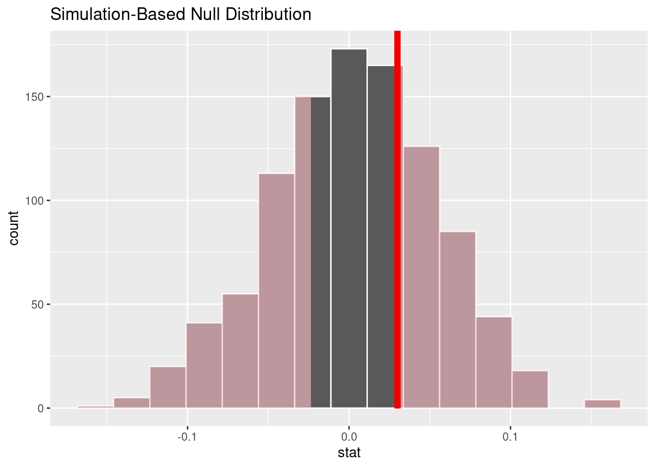
We can then calculate the point estimate, which tells us what the observed difference in average day arrests were made in male vs female perpetrators was: 0.03.
We generated the null distribution through permutation 1000 times.
# A tibble: 1 × 1
  p_value
    <dbl>
1     0.6
Due to the p-value greater than 0.05, we fail to reject the null hypothesis. There is not significant evidence to suggest there is a difference in the average day women are arrested as opposed to men.
Interpretation and Conclusions
Interpretation and Conclusions #1
An analysis of the data through summary statistics and visualizations reveals some common themes. First, men are arrested at rates much higher (4-5x) than that of women. Next, black men are arrested the most with rates double that of white hispanics (the next largest racial group). Furthermore, from our significance test, we can reject all the proposed null hypothesis and conclude that the observed differences in male vs female felony convictions, black vs. white felony convictions, and black vs white felony convictions for ‘dangerous drugs’ are all statistically significant. The difference in proportion of black people who received felony convictions for ‘dangerous drugs’ versus white people might allude to some discrimination in the criminal justice system. While nothing is definitive it should be some cause for alarm. The same can be said for the other results we observed. Are men that much more likely to be arrested for felonies than women? Are black people truly that much more likely to be arrested for felonies than white people? While that may truly be the case, there may also be some other factors at play such as over-policing certain areas, biases against certain races/genders by police, and more. One final analysis that we could do moving forward would be to directly compare rates of arrest for black women and men vs white women and men. Are black women more likely to be arrested than white women as compared to black and white men?
Interpretation and Conclusions #2
In the evaluation of significance, we rejected the null hypothesis, signifying the the proportion of females being arrested in Staten Island is different from the city-wide proportion. This raises a few additional questions. I wonder if the female population of Staten Island is also statistically different than citywide. Also, I wonder if the lower population of Staten Island can have an effect on these result. Are there any particular characteristics of Staten Island that are unique to the borough that can make this true?
Interpretation and Conclusions #3
In the evaluation of significance, we failed to reject the null hypothesis. This means that, based on the model, we can conclude that men and women tend to be arrested on the same average day during the month which implies that the rates of arrest throughout the month are similar. This is an interesting finding as women are much less likely to get arrested than men as we concluded in our first analysis. The fact that genders are arrested at same rates each day (relative to their own gender) throughout the month despite significant differences in numbers for each gender shows consistency in the policing of the city as well as criminal activity throughout the month.
Limitations
Limitations #1
There are some limitations for this study, such as the arrest data only including people who were arrested, which might not be representative of the whole population of people committing crimes; selection bias. For future analysis on our third hypothesis we could look deeper in to the broad category of “dangerous drugs”. Maybe the amount of the drug possessed, intent, or type of drug plays a role in this difference?Finally, there are also some ethical considerations, as we are dealing with attributes such as race and gender, which could reinforce stereotypes or discrimination. As touched on in the conclusion, the over policing of black people and other stereotypes likely play a role in the significant overrepresentation of black people, especially males, in the dataset.
Limitations #2
As mentioned in the conclusion, there are some uncertainties that prevent us from strongly supporting this result. One of such is that we do not know if the true proportion of female perpetrators in Staten Island is statistically different from the citywide average. The lower population of Staten Island can affect the data and provide more skewed results. We would need additional information to conduct this analysis.
Limitations #3
A major limitation for this third analysis is the fact that this data is entirely from the year 2022 with some months from 2023. Due to the nature of coming out of recent lock downs there may be some influences on trends where we see more criminal activity as more people are outside. Furthermore, having data only from one year makes it hard to cross examine other years and see if this year was an outlier. Maybe the winter months of other years have higher crime rates than non-winter months or maybe there is no difference. Being able to compare data across multiple years would be very valuable for evaluating significance of the noticed trends.
Acknowledgments
The source of our data is https://data.cityofnewyork.us/Public-Safety/NYPD-Arrest-Data-Year-to-Date-/uip8-fykc. The website is NYC Open Data and the data set itself is aggregated by the Office of Management Analysis and Planning who manually extracted the original data from hand written police reports.
A very helpful source we utilized when creating null distributions through random sampling was https://cran.r-project.org/web/packages/infer/vignettes/observed_stat_examples.html#one-numerical-one-categorical-2-levels—anova.