── Attaching packages ─────────────────────────────────────── tidyverse 1.3.2 ──
✔ ggplot2 3.4.0     ✔ dplyr   1.1.2
✔ tibble  3.2.1     ✔ stringr 1.5.0
✔ tidyr   1.2.1     ✔ forcats 0.5.2
✔ purrr   1.0.0
── Conflicts ────────────────────────────────────────── tidyverse_conflicts() ──
✖ dplyr::filter() masks stats::filter()
✖ dplyr::lag()    masks stats::lag()
── Attaching packages ────────────────────────────────────── tidymodels 1.0.0 ──

✔ broom        1.0.2     ✔ rsample      1.1.1
✔ dials        1.1.0     ✔ tune         1.1.1
✔ infer        1.0.4     ✔ workflows    1.1.2
✔ modeldata    1.0.1     ✔ workflowsets 1.0.0
✔ parsnip      1.0.3     ✔ yardstick    1.1.0
✔ recipes      1.0.6

── Conflicts ───────────────────────────────────────── tidymodels_conflicts() ──
✖ scales::discard() masks purrr::discard()
✖ dplyr::filter()   masks stats::filter()
✖ recipes::fixed()  masks stringr::fixed()
✖ dplyr::lag()      masks stats::lag()
✖ yardstick::spec() masks readr::spec()
✖ recipes::step()   masks stats::step()
• Learn how to get started at https://www.tidymodels.org/start/

Loading required package: timechange


Attaching package: 'lubridate'


The following objects are masked from 'package:base':

date, intersect, setdiff, unionPredicting NFL Team Performance
with ELO Rating, Home-Field Advantage, and QB Rating
Introduce the topic and motivation
The research topic is NFL games. For people who are not familiar with this, the NFL is the American football league founded in 1920. It comprises of 32 teams across the country that compete in 17 regular season games, and this season concludes with a single-elimination playoff bracket. In this dataset, the Elo rating system is utilized. Elo is a simple measure of team strength and performance that is calculated based on game-by-game results. This provides an accurate description of a team’s rating before and after every game they have played.
Introduce the data
Research question: Does having the home field really give the NYG team an advantage? Do other variables such as quarterback rating or overall team rating affect this advantage?
We analyzed the NFL Elo dataset provided by FiveThirtyEight, which contains historical data on NFL games and Elo ratings for each team. The dataset covers games from the beginning of the league in 1920 through the 2021 season.
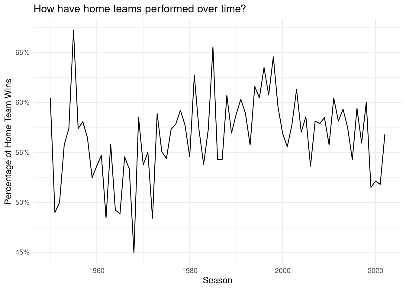
Highlights from EDA
Data Cleaning:
nfl_data <- read_csv("data/nfl_elo.csv")Rows: 17379 Columns: 33
── Column specification ────────────────────────────────────────────────────────
Delimiter: ","
chr (5): playoff, team1, team2, qb1, qb2
dbl (27): season, neutral, elo1_pre, elo2_pre, elo_prob1, elo_prob2, elo1_p...
date (1): date
ℹ Use `spec()` to retrieve the full column specification for this data.
ℹ Specify the column types or set `show_col_types = FALSE` to quiet this message.active_teams <- c(
"ARI", "ATL", "BAL", "BUF", "CAR", "CHI", "CIN",
"CLE", "DAL", "DEN", "DET", "GB", "HOU", "IND",
"JAX", "KC", "MIA", "MIN", "NE", "NO", "NYG",
"NYJ", "LV", "PHI", "PIT", "LAC", "SF", "SEA",
"LAR", "TB", "TEN", "WAS"
)
nfl_data_clean <- nfl_data |>
mutate(
winning_team = if_else(score1 > score2, team1, team2),
playoff = if_else(is.na(playoff), "R", playoff),
home_win = if_else(winning_team == team1, TRUE, FALSE)
) |>
group_by(team1) |>
filter(season >= 1950, team1 %in% active_teams, team2 %in% active_teams) |>
arrange(team1)
select(nfl_data_clean, -total_rating, -importance)# A tibble: 13,056 × 33
# Groups: team1 [30]
date season neutral playoff team1 team2 elo1_pre elo2_pre elo_prob1
<date> <dbl> <dbl> <chr> <chr> <chr> <dbl> <dbl> <dbl>
1 1950-09-24 1950 0 R ARI PHI 1554. 1632. 0.482
2 1950-10-29 1950 0 R ARI NYG 1525. 1529. 0.587
3 1950-11-05 1950 0 R ARI CLE 1547. 1679. 0.405
4 1950-11-23 1950 0 R ARI PIT 1536. 1504. 0.636
5 1950-12-03 1950 0 R ARI CHI 1503. 1668. 0.360
6 1951-09-30 1951 0 R ARI PHI 1506. 1585. 0.479
7 1951-10-07 1951 0 R ARI CHI 1492. 1596. 0.444
8 1951-10-28 1951 0 R ARI PIT 1489. 1467. 0.623
9 1951-11-04 1951 0 R ARI CLE 1454. 1678. 0.286
10 1951-11-25 1951 0 R ARI NYG 1456. 1601. 0.387
# ℹ 13,046 more rows
# ℹ 24 more variables: elo_prob2 <dbl>, elo1_post <dbl>, elo2_post <dbl>,
# qbelo1_pre <dbl>, qbelo2_pre <dbl>, qb1 <chr>, qb2 <chr>,
# qb1_value_pre <dbl>, qb2_value_pre <dbl>, qb1_adj <dbl>, qb2_adj <dbl>,
# qbelo_prob1 <dbl>, qbelo_prob2 <dbl>, qb1_game_value <dbl>,
# qb2_game_value <dbl>, qb1_value_post <dbl>, qb2_value_post <dbl>,
# qbelo1_post <dbl>, qbelo2_post <dbl>, score1 <dbl>, score2 <dbl>, …write.csv(nfl_data_clean, file = "data/nfl_data_clean.csv") Exploratory data analysis:
Inference/modeling/other analysis #1
Home-Field Advantage Analysis
Call:
glm(formula = glm_win ~ glm_home, family = binomial, data = nfl_data_clean_NYG)

Deviance Residuals:
   Min      1Q  Median      3Q     Max
-1.218  -1.091  -1.091   1.137   1.266

Coefficients:
            Estimate Std. Error z value Pr(>|z|)
(Intercept) -0.20618    0.09206  -2.240   0.0251 *
glm_home     0.30109    0.12939   2.327   0.0200 *
---
Signif. codes:  0 '***' 0.001 '**' 0.01 '*' 0.05 '.' 0.1 ' ' 1

(Dispersion parameter for binomial family taken to be 1)

    Null deviance: 1332.9  on 961  degrees of freedom
Residual deviance: 1327.5  on 960  degrees of freedom
AIC: 1331.5

Number of Fisher Scoring iterations: 3- Models chances of winning based on home field for New York Giants
- Data was narrowed down to NYG and NYJ due to team preferences and abundance of data for these teams
Inference/modeling/other analysis #2
Hypothesis Test + Prediction # 1
Response: win (factor)
Explanatory: home (factor)
# A tibble: 1 × 1
    stat
   <dbl>
1 0.0751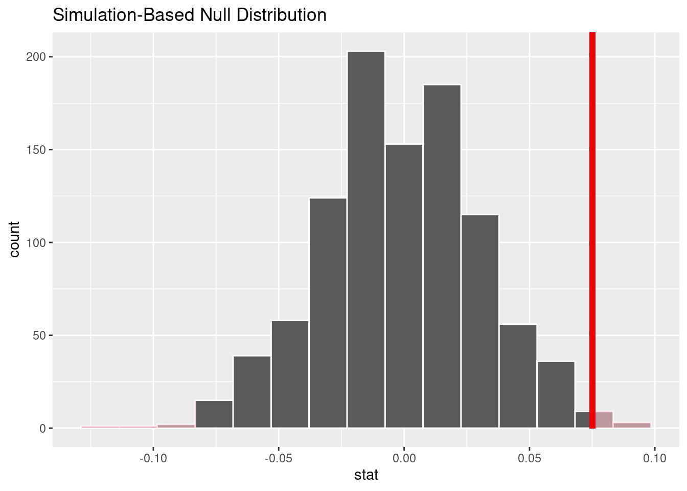
# A tibble: 1 × 1
  p_value
    <dbl>
1 0.02- For NYG data, since the p_value < 0.05, then this is statistically significant and we reject the null hypothesis. There is enough evidence to conclude that the probability of team “NYG” winning a home game is not equal to the probability of it winning an away game.
Hypothesis Test + Prediction # 2
Call:
glm(formula = glm_win ~ home + giants_elo_score + giants_qb_score,
    data = nfl_data_clean_NYG)

Deviance Residuals:
    Min       1Q   Median       3Q      Max
-0.8123  -0.2575  -0.1762   0.2691   0.8238

Coefficients:
                     Estimate Std. Error t value Pr(>|t|)
(Intercept)           0.17617    0.02336   7.541 1.08e-13 ***
homeyes               0.08134    0.02687   3.027  0.00254 **
giants_elo_scoreTRUE  0.07628    0.07277   1.048  0.29476
giants_qb_scoreTRUE   0.47848    0.07276   6.576 7.92e-11 ***
---
Signif. codes:  0 '***' 0.001 '**' 0.01 '*' 0.05 '.' 0.1 ' ' 1

(Dispersion parameter for gaussian family taken to be 0.173556)

    Null deviance: 240.32  on 961  degrees of freedom
Residual deviance: 166.27  on 958  degrees of freedom
AIC: 1051.3

Number of Fisher Scoring iterations: 2
1
0.8122712 Model was combined with elo score and qb score to make an accurate prediction for the game
Model showed ~ 81% chance of winning
Conclusions + future work
Conclusion: Home-field advantage is truly grounded in statistical evidence
Additionally, the notion that the quarterback is the most important player or the “field general” fails to be confirmed.
While qb rating does predict wins, overall team rating(defense, skill players etc) is a better predictor.
In the future:
Analyze more NFL teams to make more generalizations regarding the entire league
Analyze more variables that can impact the game’s outcome, such as stakes, weather, etc