Predicting NFL Team Performance with ELO Rating, Home-Field Advantage, and QB Rating
Report
Introduction
In this project, we will be evaluating NFL data since 1920 using 538’s “Complete History of the NFL” dataset. This data was chosen as several members of the group are football fans, and today in sports, understanding who is going to win a specific game is extremely important in activities such as sports betting. Our research question is: Does having the home field really give the New York Giants (NYG) or Jets (NYJ) an advantage? Is this advantage more or less pronounced in the playoffs? Overall, throughout our research, we found the advantage to be statistically significant, and this effect is enhanced by overall team strength at the time of the game, and equally enhanced by the quarterback’s individual rating. Therefore, the following analyses provide greater insight into predicting NFL game outcomes over time.
Research question: Does having the home field really give the NYG team an advantage? Is this advantage different or more pronounced in the playoffs?
Data description
We analyzed the NFL Elo dataset provided by FiveThirtyEight, which contains historical data on NFL games and Elo ratings for each team. The dataset covers games from the beginning of the league in 1920 through the 2021 season. Elo ratings are a measure of a team’s strength and are used to predict the outcome of games based on each team’s relative skill level.
In addition to the Elo ratings, the dataset includes information about the game date, season, teams involved, where the game is played, playoff status, and the actual scores for each team. The dataset also contains advanced statistics such as quarterback Elo ratings.
Our focus is to analyze how a team’s Elo rating can predict their winning probability during the regular season, playoffs, and Super Bowl. In doing so, we will consider additional factors such as the location of the game and the quarterback ratings. By incorporating these elements, we aim to gain a deeper understanding of the factors influencing game outcomes, allowing us to draw more informed and nuanced conclusions.
Data analysis
Home-Field Advantage Analysis
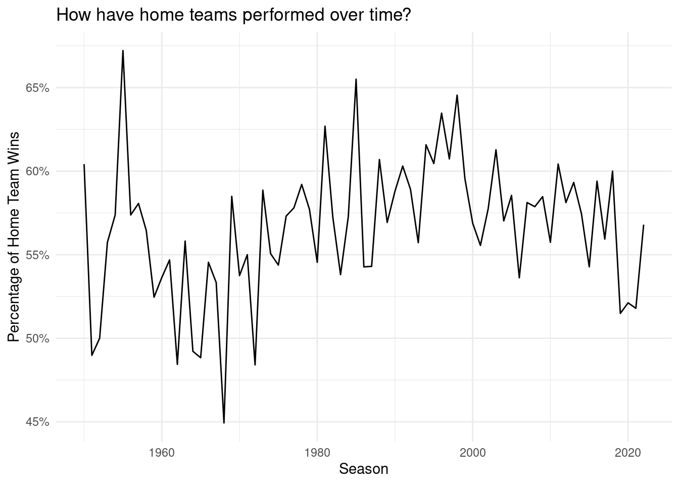
The home team performance fluctuates over time. The fluctuation is more obvious before 1980. After 1980, it’s more stable, fluctuating from 52% to 65%. It shows the home team has an advantage.
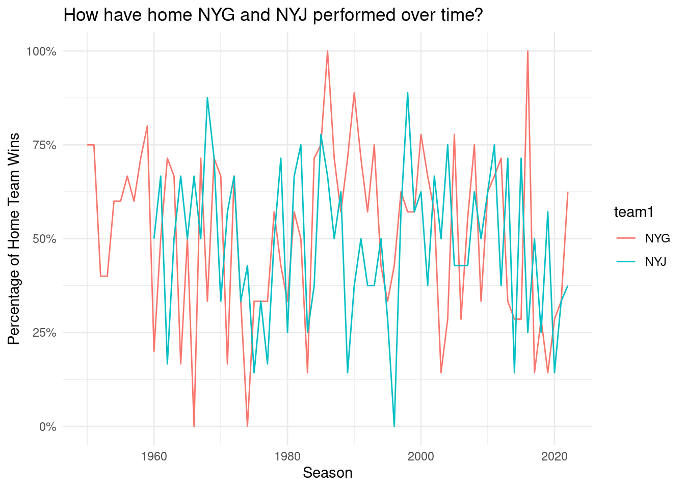
Overall, these two graphs show both overall home-field winning percentages as well as home-field winning percentages for only NYJ and NYG. As shown, winning percentages are relatively erratic over time, yet stabilize to about 60% in the year 2020.
NYG Team Regression Analysis:
Call:
glm(formula = glm_win ~ glm_home, family = binomial, data = nfl_data_clean_NYG)

Deviance Residuals:
   Min      1Q  Median      3Q     Max
-1.218  -1.091  -1.091   1.137   1.266

Coefficients:
            Estimate Std. Error z value Pr(>|z|)
(Intercept) -0.20618    0.09206  -2.240   0.0251 *
glm_home     0.30109    0.12939   2.327   0.0200 *
---
Signif. codes:  0 '***' 0.001 '**' 0.01 '*' 0.05 '.' 0.1 ' ' 1

(Dispersion parameter for binomial family taken to be 1)

    Null deviance: 1332.9  on 961  degrees of freedom
Residual deviance: 1327.5  on 960  degrees of freedom
AIC: 1331.5

Number of Fisher Scoring iterations: 3
NYJ Team Regression Analysis:
Call:
glm(formula = glm_win ~ glm_home, family = binomial, data = nfl_data_clean_NYJ)

Deviance Residuals:
   Min      1Q  Median      3Q     Max
-1.155  -1.155  -1.005   1.200   1.360

Coefficients:
            Estimate Std. Error z value Pr(>|z|)
(Intercept) -0.41970    0.09439  -4.446 8.73e-06 ***
glm_home     0.36774    0.13257   2.774  0.00554 **
---
Signif. codes:  0 '***' 0.001 '**' 0.01 '*' 0.05 '.' 0.1 ' ' 1

(Dispersion parameter for binomial family taken to be 1)

    Null deviance: 1277.8  on 930  degrees of freedom
Residual deviance: 1270.1  on 929  degrees of freedom
AIC: 1274.1

Number of Fisher Scoring iterations: 4
Analysis of Quarterback ELO Scores vs. Overall Team Scores
# A tibble: 2 × 5
  term                estimate std.error statistic  p.value
  <chr>                  <dbl>     <dbl>     <dbl>    <dbl>
1 (Intercept)            -1.26     0.108     -11.7 2.09e-31
2 giants_qb_scoreTRUE     2.47     0.154      16.0 1.78e-57
# A tibble: 1 × 8
null.deviance df.null logLik AIC BIC deviance df.residual nobs
<dbl> <int> <dbl> <dbl> <dbl> <dbl> <int> <int>
1 1333. 961 -513. 1031. 1041. 1027. 960 962# A tibble: 2 × 5
term estimate std.error statistic p.value
<chr> <dbl> <dbl> <dbl> <dbl>
1 (Intercept) -1.18 0.106 -11.2 6.56e-29
2 giants_elo_scoreTRUE 2.30 0.151 15.3 1.62e-52# A tibble: 1 × 8
null.deviance df.null logLik AIC BIC deviance df.residual nobs
<dbl> <int> <dbl> <dbl> <dbl> <dbl> <int> <int>
1 1333. 961 -530. 1064. 1074. 1060. 960 962Overall, these two models provided significant insight into whether the New York Giants were going to win a game or not. Therefore, the below model combines the three variables(home field, qb elo rating, and overall team rating) to predict whether the Giants would win a game or not.
Call:
glm(formula = glm_win ~ home + giants_elo_score + giants_qb_score,
    data = nfl_data_clean_NYG)

Deviance Residuals:
    Min       1Q   Median       3Q      Max
-0.8123  -0.2575  -0.1762   0.2691   0.8238

Coefficients:
                     Estimate Std. Error t value Pr(>|t|)
(Intercept)           0.17617    0.02336   7.541 1.08e-13 ***
homeyes               0.08134    0.02687   3.027  0.00254 **
giants_elo_scoreTRUE  0.07628    0.07277   1.048  0.29476
giants_qb_scoreTRUE   0.47848    0.07276   6.576 7.92e-11 ***
---
Signif. codes:  0 '***' 0.001 '**' 0.01 '*' 0.05 '.' 0.1 ' ' 1

(Dispersion parameter for gaussian family taken to be 0.173556)

    Null deviance: 240.32  on 961  degrees of freedom
Residual deviance: 166.27  on 958  degrees of freedom
AIC: 1051.3

Number of Fisher Scoring iterations: 2
1
0.8122712 From the model above, in a given game in which the Giants are home, have a better quarterback than the other team, and have a better overall team than their opponent, their chances of winning are approximately equal to 0.81, much higher than the league average. While this model is only specific to the Giants, they were chosen in part due to their abundance of data in the data set. Their games date back to 1920, thus providing ample data to work with and model winning percentages.
Evaluation of significance
After selecting some teams such as the New York Giants and New York Jets, we tested hypotheses for each one. We will then calculate the p-value to test the significance and interpret it in the context. Confidence intervals will be constructed if needed.
Hypothesis tests 1:
Null hypothesis: The probability of team “NYG” winning a home game is equal to the probability of it winning an away game.
Alternative hypothesis: The probability of team “NYG” winning a home game is not equal to the probability of it winning an away game. \[
H_0: p_h - p_a = 0
\]
\[ H_A: p_h - p_ a \neq 0 \]
Response: win (factor)
Explanatory: home (factor)
# A tibble: 1 × 1
    stat
   <dbl>
1 0.0751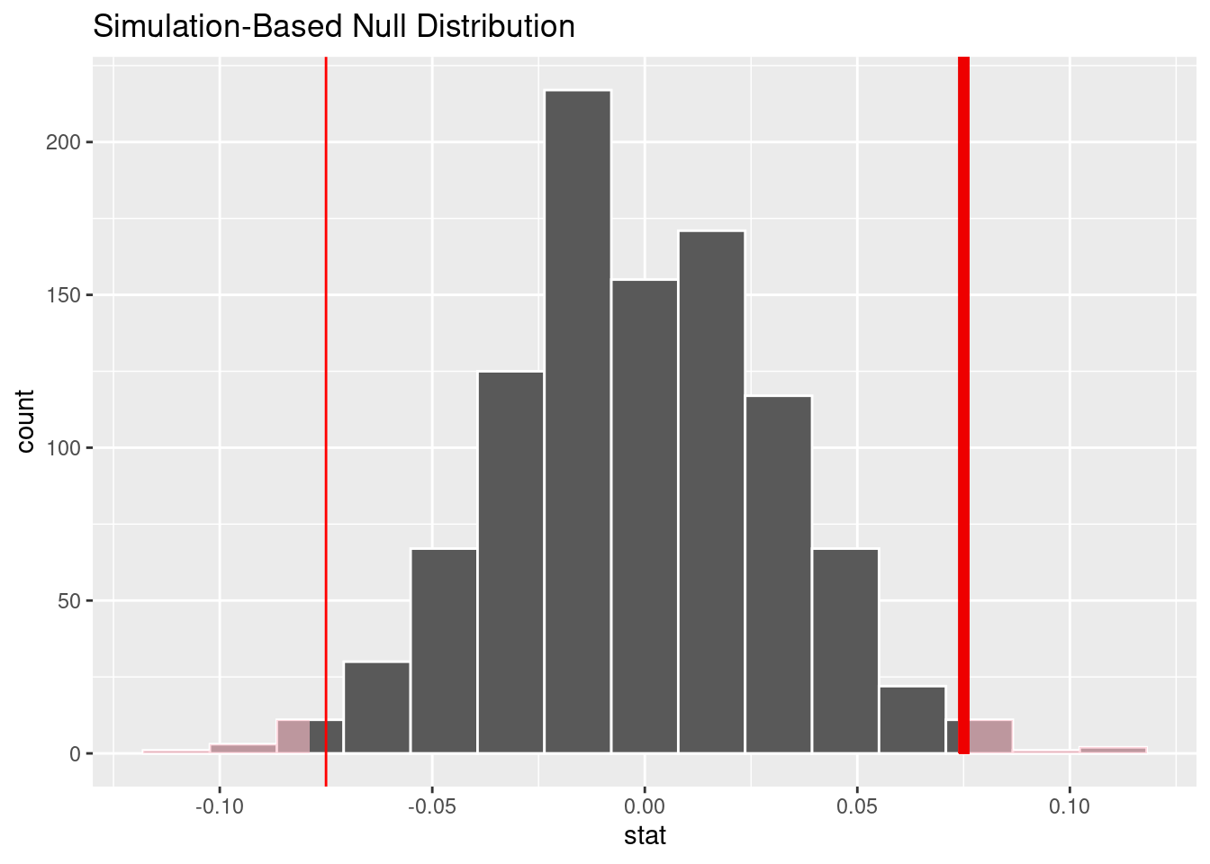
# A tibble: 1 × 1
  p_value
    <dbl>
1   0.014
Hypothesis tests 2:
H_0: The probability of team “NYJ” winning a home game is equal to the probability of it winning an away game.
H_A: The probability of team “NYJ” winning a home game is not equal to the probability of it winning an away game. \[
H_0: p_h - p_a = 0
\]
\[ H_A: p_h - p_ a \neq 0 \]
Response: win (factor)
Explanatory: home (factor)
# A tibble: 1 × 1
    stat
   <dbl>
1 0.0904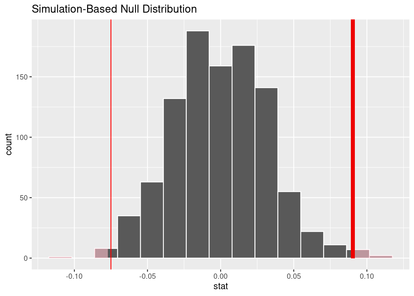
# A tibble: 1 × 1
  p_value
    <dbl>
1   0.012
Interpretation and conclusions
For NYG data, since the p_value < 0.05, then this is statistically significant and we reject the null hypothesis. There is enough evidence to conclude that the probability of team “NYG” winning a home game is not equal to the probability of it winning an away game.
For NYJ data, since the p_value < 0.05, then this is statistically significant and we reject the null hypothesis. There is enough evidence to conclude that the probability of team “NYJ” winning a home game is not equal to the probability of it winning an away game.
In conclusion, there is a home team advantage in the game. In real life, it can be applied to decision-making and game planning to ensure fairness in the game.
Limitations
The dataset does include ELO values as well as other relevant information needed to address the majority of the research questions. One of the research questions pertains to finding the contribution of a quarterback’s ELO score to a team’s overall ELO rating. It is easier to establish a correlative relationship and more difficult to use the data to prove the extent of contribution. In this way, it is challenging to precisely answer the research question with the data. Otherwise, it seems plausible to address the remaining research questions with the dataset.
The study also has another limitation on the team sample variety. Due to time limit and data size, We specifically evaluated team NYJ and NYG. It can be more comprehensive by evaluating more teams.
Acknowledgments
Dataset source: FiveThirtyEight https://projects.fivethirtyeight.com/complete-history-of-the-nfl/