Introduce the topic and motivation
Our project is focused on exploring the relationship between different variables amongst the 100 most popular movies (from iMDB) for each year from 2003-2022. The research questions we are exploring here are:
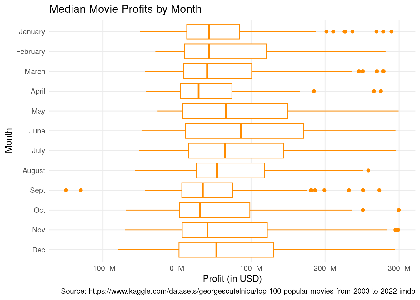
- Which release dates see the greatest profits?
- How strong is the relationship between a film’s release year and income versus its iMDB rating?
Introduce the data
100 most popular movies for each year from 2003-2022
1989 (why not 2000?) rows and 13 columns
Movie title, iMDB rating, year of release, month of release, budget, income, etc.
Each row represents a unique film that has all the above data on iMBD
Q1 – Highlights from EDA
Attaching package: 'dplyr'
The following objects are masked from 'package:stats':

    filter, lag
The following objects are masked from 'package:base':

    intersect, setdiff, setequal, union
── Attaching packages ─────────────────────────────────────── tidyverse 1.3.2 ──
✔ ggplot2 3.4.0     ✔ purrr   1.0.0
✔ tibble  3.2.1     ✔ stringr 1.5.0
✔ tidyr   1.2.1     ✔ forcats 0.5.2
── Conflicts ────────────────────────────────────────── tidyverse_conflicts() ──
✖ dplyr::filter() masks stats::filter()
✖ dplyr::lag()    masks stats::lag()
── Attaching packages ────────────────────────────────────── tidymodels 1.0.0 ──

✔ broom        1.0.2     ✔ rsample      1.1.1
✔ dials        1.1.0     ✔ tune         1.1.1
✔ infer        1.0.4     ✔ workflows    1.1.2
✔ modeldata    1.0.1     ✔ workflowsets 1.0.0
✔ parsnip      1.0.3     ✔ yardstick    1.1.0
✔ recipes      1.0.6

── Conflicts ───────────────────────────────────────── tidymodels_conflicts() ──
✖ scales::discard() masks purrr::discard()
✖ dplyr::filter()   masks stats::filter()
✖ recipes::fixed()  masks stringr::fixed()
✖ dplyr::lag()      masks stats::lag()
✖ yardstick::spec() masks readr::spec()
✖ recipes::step()   masks stats::step()
• Search for functions across packages at https://www.tidymodels.org/find/

Rows: 2000 Columns: 13
── Column specification ────────────────────────────────────────────────────────
Delimiter: ","
chr (11): Title, Month, Certificate, Runtime, Directors, Stars, Genre, Filmi...
dbl  (2): Rating, Year

ℹ Use `spec()` to retrieve the full column specification for this data.
ℹ Specify the column types or set `show_col_types = FALSE` to quiet this message.
Q1 – Inference/modeling/other analysis
Warning: Please be cautious in reporting a p-value of 0. This result is an
approximation based on the number of `reps` chosen in the `generate()` step. See
`?get_p_value()` for more information.
# A tibble: 1 × 1
  p_value
    <dbl>
1       0
\[
p-value=0<0.05=\alpha
\]
We reject the null hypothesis in favor of the alternate hypothesis.
Therefore, the data provides evidence that the there is a difference in profits between favorable and unfavorable months.
Q1 – Inference/modeling/other analysis
# A tibble: 1 × 2
   lower_ci   upper_ci
      <dbl>      <dbl>
1 16356012. 135972444.
We are 95% confident that the true mean profit of favorable months is between ~16 million USD to ~136 million USD higher than the profit for unfavorable months, on average.
If we were to simulate this again, at least 95% of these intervals will contain the true mean.
Q1 – Conclusions/Future Work
Observation: Movies released in favorable months (May, June, July, December) have a higher average profit then those released in unfavorable months (all other months).
Inference: We can expect movies released in May, June, July, Dec to earn a higher profit (on average) as opposed to movies that released in other months.
Support: Confidence interval and p-value (which showed us that there is a statistically significant difference in profits between favorable and unfavorable release months).
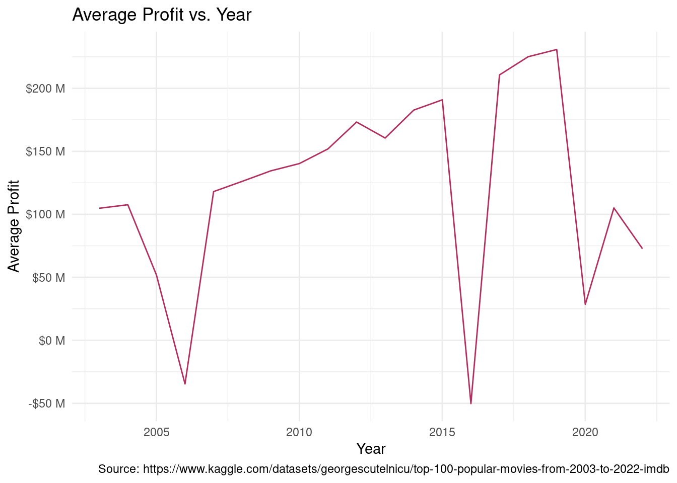
- Small drop around 2020 (can be attributed to COVID-19)
- Future work can do a detailed analysis of profits for release years to find more trends and explore the cause for this dips
Q2 – Highlights from EDA
Warning: There was 1 warning in `mutate()`.
ℹ In argument: `income = parse_number(income)`.
Caused by warning:
! 145 parsing failures.
row col expected  actual
  6  -- a number Unknown
 16  -- a number Unknown
 17  -- a number Unknown
 18  -- a number Unknown
 19  -- a number Unknown
... ... ........ .......
See problems(...) for more details.
Q2 – Inference/modeling/other analysis
# A tibble: 3 × 5
  term         estimate std.error statistic  p.value
  <chr>           <dbl>     <dbl>     <dbl>    <dbl>
1 (Intercept) -8.44e- 1  7.30e+ 0    -0.116 9.08e- 1
2 year         3.70e- 3  3.63e- 3     1.02  3.09e- 1
3 income       5.84e-10  7.34e-11     7.96  3.09e-15
\[ \begin{split} \widehat{Rating} = -8.440238*10^{-1} + 3.696143*10^{-3} \times Year \\ + 5.842187*10^{-10} \times Income \end{split} \]
When year and income = 0, expected rating is -0.844.
Expected rating increases by 0.0037 for every additional year and by 5.842187*10-10 for every additional dollar.
Q2 – Inference/modeling/other analysis
# A tibble: 1 × 1
       r
   <dbl>
1 0.0317
# A tibble: 1 × 1
      r
  <dbl>
1 0.183
- Correlation between release year and iMDB rating is negligible because r ~ 0, and income has a weakly positive relationship with rating (r = 0.1829604).
# A tibble: 1 × 2
  lower_ci upper_ci
     <dbl>    <dbl>
1   0.0938    0.256
- CI for blockbuster movies (income of at least $100,000,000) vs. non-blockbuster movies.
Q2 – Conclusions/Future Work
Observation: Movies with high box office incomes tend to earn higher iMDB ratings.
Inference: We can expect movies earning at least $100,000,000 at the box office to have higher iMDB ratings than those earning less than $100,000,000.
Support: Confidence interval, which showed us that the true mean difference between blockbusters and non-blockbusters is probably positive.
Could explore further by . . .
References
The data that we used was from Kaggle, by a user with the username GEORGE SCUTELNICU (https://www.kaggle.com/datasets/georgescutelnicu/top-100-popular-movies-from-2003-to-2022-imdb).


