Team Elegant Evee
Report on IMDb Ratings (2003 to 2022)
Introduction
To begin, we will briefly discuss the source of our data, namely a dataset on Kaggle (https://www.kaggle.com/datasets/georgescutelnicu/top-100-popular-movies-from-2003-to-2022-IMDb) submitted by George Scutelnicu. The data were collected from 2003 to 2022, and the dataset’s author scraped the top 100 most popular movies during this ninteen-year period through IMDb, a movie rating website. In all, the dataset contains film information like movies’ ratings, release years, runtimes, filming locations, and more—a total of 13 columns and 1989 rows.
Given this dataset, our project is focused on exploring the relationship between different variables in the dataset described above. To this end, we propose two research questions, namely: “Which release dates see the greatest profits?” and”What is the relationship between a film’s release year and income versus its IMDb rating?”
The context of our work is essentially to look at film profits and how they evolve over time, and we apply techniques like bootstrapping and hypothesis testing to answer these two research questions. Ultimately, we find that film profits have generally risen annually, albeit with dips in recent years—potentially due to economic factors like recessions and COVID-19—and we further find that the months that see the greatest profits are May, June, July, and, December. Lastly, we present evidence that movies with high box office incomes tend to earn higher IMDb ratings and that film quality has not markedly declined over time. Our submission challenges conventional wisdom about films and provides new intuitions that may help to explain post-pandemic trends.
Data Description
Before analyzing the data, we will briefly describe our dataset using questions inspired by Gebru et al. (2018).
What are the observations (rows) and the attributes (columns)?
The attributes or variables in our dataset represent film details, namely movie title, IMDb rating, year of release, month of release, certificate, runtime, director(s), stars, genre(s), filming location, budget, income, and country of origin. Each observation or row represents a unique film that has all the above data on iMBD. Note that this data set contains the 100 most popular movies for each year from 2003-2022.
Why was this dataset created?
This data was created on Kaggle for use for exploratory data analysis for anyone on the internet—the intention is to keep records of the most popular movies across time and motivate discussion about what makes films successful.
Who funded the creation of the dataset?
The dataset was voluntarily created for Kaggle by a user with the username GEORGE SCUTELNICU.
What processes might have influenced what data was observed and recorded and what was not?
Since the data was web scraped from the IMDb website, IMDb’s policies are the primary influence on what data was observed and recorded. It is possible that certain kinds of movies or certain controversial directors or stars are forbidden from the ranking list—or that their search algorithm was biased against certain types of movies. Given that ranking methods and moderation affect public-facing information, web-scraped datasets are consequently affected as well.
What preprocessing was done, and how did the data come to be in the form that you are using?
To preprocess the data, GEORGE SCUTELNICU on Kaggle mainly conducted web scraping. To turn scraped data into usable values, the author likely conducted significant cleaning to produce the eventual thirteen-column dataset, including deliminating films with multiple genres with commas. However, no reproducibility information accompanies the dataset, so we are unable to provide more specific details.
If people are involved, were they aware of the data collection and if so, what purpose did they expect the data to be used for?
This data was collected intentionally. The purpose listed on the website was for exploratory data analysis for anyone on the internet who came across the data set. Although IMDb users were not aware of the data collection for Kaggle, the dataset was sourced from web-scraped IMDb data—information which is inherently crowdsourced and where no personally identifiable information is revealed.
Is the dataset self-contained, or does it link to or otherwise rely on external resources (e.g., websites, tweets, other datasets)?
A quick look at the data shows that it is indeed self-contained. None of the entries in the dataset refer to any other website or any other dataset. All entries are alphanumeric and local.
Does the dataset contain data that might be considered confidential?
No, the dataset does not consider any data that is considered confidential. Individual submissions on IMDb, a public-facing website, are only included in the dataset in the form of aggregated film rating scores. All other information concerns logistical and financial information about films that is already public knowledge.
Has the dataset been used for any tasks already?
Since the dataset is available for public use on Kaggle, the data has likely been used for tasks by other individuals, as the dataset has been downloaded 3033 times, as of the time of writing.
Is there a repository that links to any or all papers or systems that use the dataset?
Yes, the link to the Kaggle site where this dataset is available (https://www.kaggle.com/datasets/georgescutelnicu/top-100-popular-movies-from-2003-to-2022-IMDb) contains information on which users and how many users have viewed and used this dataset before. The “Dataset Notebooks” section (https://www.kaggle.com/datasets/georgescutelnicu/top-100-popular-movies-from-2003-to-2022-IMDb/code) provides information on which current Kaggle members use the data.
Question 1
1.1. Data analysis
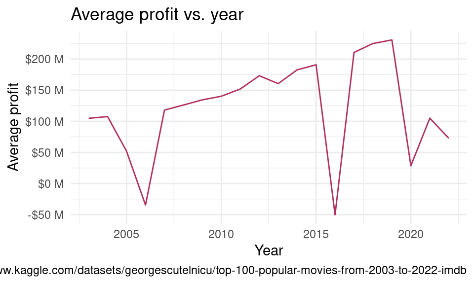
We can see that the average profit over the last few decades has been on the rise, except for 2006 and 2016 which seem to have had a significant decrease in profit (these are actually losses) and a dip in 2020 as well (which we know can be attributed to COVID) and the years after.
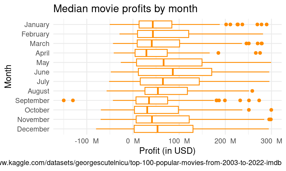
According to the plot, the month with the highest median is June, and the month with the lowest median is April. Additionally, summer and winter seasons usually have higher profits than fall and spring releases, and most of the outliers are high-profit movies, making the distribution right-skewed. This boxplot provides us with the median profits per month, which is helpful, as the median is unaffected by the skew.
Please note that the data has been filtered to only represent only profits that are greater than -$150 million and less than $300 million dollars. This is because the outliers outside of this range are so extreme that we cannot see the boxplots clearly.
# A tibble: 1 × 2
        mean         sd
       <dbl>      <dbl>
1 123390922. 541501058.
The mean for the profit of all the movies in our dataset is $123,390,922 and the standard deviation is $541,501,058.
# A tibble: 2 × 5
  term            estimate   std.error statistic p.value
  <chr>              <dbl>       <dbl>     <dbl>   <dbl>
1 (Intercept) -5059000671. 6125641083.    -0.826   0.420
2 year            2574177.    3043784.     0.846   0.409
The linear model for the relationship between the average profit and the month is as follows.
\[ \widehat{profit} = -5,059,000,671 + 2,574,177 \times Year \]
There is a nonsensical interpretation of the y-intercept, given that year = 0 does not make sense, so we will not analyse the intercept for our purposes. We can, however, claim that with each additional year, the expected profit increases by $2.574 million dollars.
# A tibble: 12 × 5
   term             estimate std.error statistic p.value
   <chr>               <dbl>     <dbl>     <dbl>   <dbl>
 1 (Intercept)     73801925.       NaN       NaN     NaN
 2 monthFebruary   34201689.       NaN       NaN     NaN
 3 monthMarch     -64665732.       NaN       NaN     NaN
 4 monthApril      62583941.       NaN       NaN     NaN
 5 monthMay       191963242.       NaN       NaN     NaN
 6 monthJune       68571484.       NaN       NaN     NaN
 7 monthJuly       31427202.       NaN       NaN     NaN
 8 monthAugust     18888267.       NaN       NaN     NaN
 9 monthSeptember  -8630989.       NaN       NaN     NaN
10 monthOctober    12568416.       NaN       NaN     NaN
11 monthNovember   89048875.       NaN       NaN     NaN
12 monthDecember  117157336.       NaN       NaN     NaN
The linear model for the relationship between the average profit and the month is:
\[ \begin{aligned} \widehat{profit} = 73,801,925 +\\ 34,201,689 \times isFebruary +\\ -64,665,732 \times isMarch + \\ 62,583,941 \times isApril + \\ 191,963,242 \times isMay + \\ 68,571,484 \times isJune + \\ 31,427,202 \times isJuly + \\ 18,888,267 \times isAugust + \\ -8,630,989 \times isSeptember + \\ 12,568,416 \times isOctober + \\ 89,048,875 \times isNovember + \\ 117,157,336 \times isDecember \end{aligned} \]
We interpret the y-intercept to be the expected profit on average in the month of January. We can see that the lowest profit is in March (as shown by our graphs above) and is about 73.8 - 64.7 = $9.1 million dollars whereas the biggest profit is in May (also shown by our graphs) and is 73.8 + 192.0 = $265.8 million dollars. We can read each coefficient with a month to be the expected increase in profit, on average, compared to that of January.
1.2. Evaluation of significance
The null hypothesis is \(\mu_1 - \mu_2 = 0\), where \(\mu_1\) represents the mean profit of the favorable months (December, May, June, and July), and \(\mu_2\) represents the mean profit of the non-favorable months (Jan, Feb, Mar, Apr, Aug, Sept, Oct, Nov). This means that there is no difference in the mean profits of favorable vs unfavorable months.
The alternate hypothesis is \(\mu_1 - \mu_2 \not= 0\), where \(\mu_1\) represents the mean profit of the favorable months (December, May, June, and July), and \(\mu_2\) represents the mean profit of the non-favorable months (Jan, Feb, Mar, Apr, Aug, Sept, Oct, Nov). This means that there is a difference in the mean profits of favorable vs unfavorable months.
# A tibble: 2 × 2
  favored_months mean_favored
  <fct>                 <dbl>
1 unfavored         94681815.
2 favored          174788321.
# A tibble: 1 × 1
p_value
<dbl>
1 0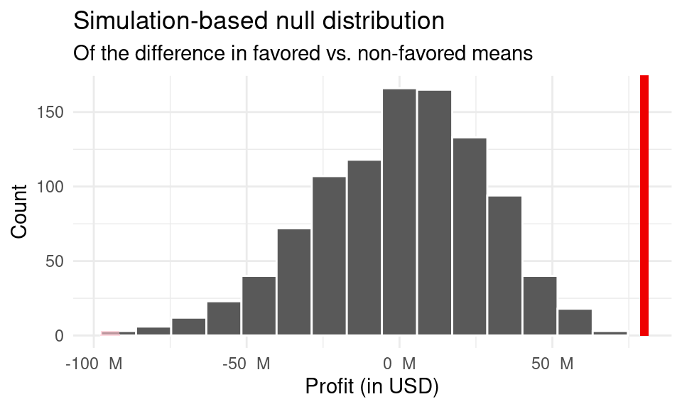
# A tibble: 1 × 2
   lower_ci   upper_ci
      <dbl>      <dbl>
1 16356012. 135972444.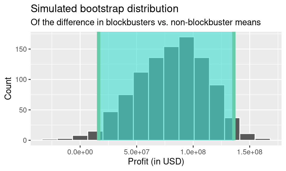
1.3. Interpretation and conclusions
Since the p-value of 0 is smaller than a significance level of 0.05, we reject the null hypothesis in favor of the alternate hypothesis. Therefore, the data provide evidence that there exists a difference in profits between favorable and unfavorable months. This is also the reasonable logical conclusion we would arrive at looking at the graphs above.
Based on the confidence interval, we are 95% confident that the true mean profit of favorable months is between 16,356,012 to 135,972,444 USD higher than the profit for unfavorable months, on average. In essence, if we were to simulate this again, at least 95% of these intervals would theoretically contain the true mean. Since this interval does not include any negative numbers, we can be assured that there exists a positive difference in the true difference in profit between the favorable and unfavorable months. Thus, we can conclude that the months that are favorable (December, May, June, and July) have a higher average profit than months that are unfavorable (Jan, Feb, Mar, Apr, Aug, Sept, Oct, Nov). This conclusion is supported by the significant range in the confidence interval, as well as the p-value, which highlighted that there was definitely a difference in profits between favorable and unfavorable release months.
In addition, it makes sense for us to have negative values because some unprofitable movies are common. Going into this, we can see that based on the median movie profits by month, summer months (May June, July) as well as December have the highest median profits compared to other months, further highlighting how our prediction that the most favorable times to release movies would be in May, June, July, and December. In addition, we can see that for the other months that aren’t favorable, the medians are generally lower and have lower profits overall. We can infer that the summer months and December would do particularly well because more students and employees have breaks and days off, allowing for time to watch movies. Given that people are busier during unfavorable months, there are usually larger losses. Thus, if one were to release a movie, based on our conclusion, it would make the most profits in May, June, July, and December.
Question 2
2.1. Data analysis
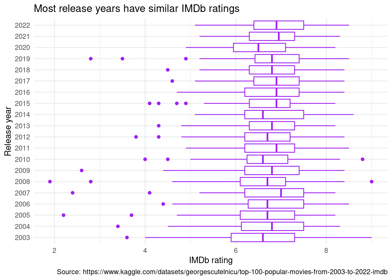
Firstly, based on this boxplot visualization, the median IMDb rating for the most popular movies has not changed much over the past two decades—the center line within each box remains between a rating 6 and 7 across release years. However, the spread of ratings has decreased slightly over time, given that the whiskers, which represent the interquartile range, have narrowed noticeable from 2003 to 2022. Lastly, most outliers are for movies with abnormally low ratings, suggesting left-skewed ratings distribution for most years, but 2020-2022 have no outliers at all. One possible explanation for this phenomenon is that, given pandemic, attending movies was a more difficult task, so fewer people made time to watch unpopular movies in the first place.
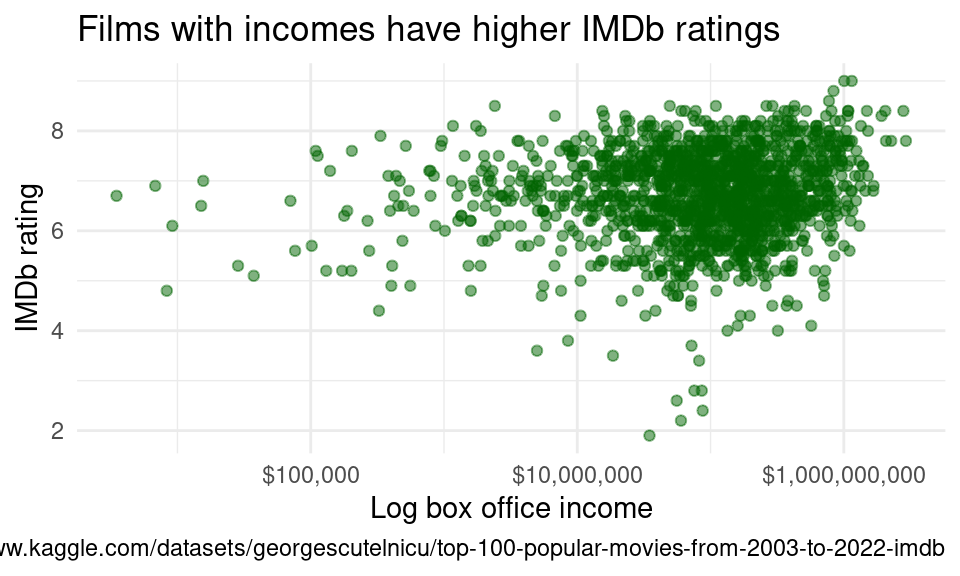
Here, we can see that the points are clustered in the top-right portion of the graph and form a somewhat elliptical cloud. On face, one might think that no noticeable relationship exists between a film’s income and IMDb. However, upon further inspection, there appears to be a weakly positive relationship between these two variables, which means that a higher box office income is associated with a higher IMDb rating. Additionally, the relationship between box office income and IMDb rating appears to be somewhat linear—the sparse points mask this relationship somewhat, but the relationship becomes clearer where the points are dense. Our correlation analysis in following sections further confirms the existence of a relationship between these variables, and the general linearity of our data gives us license to fit an ordinary least squares model.
# A tibble: 3 × 5
  term         estimate std.error statistic  p.value
  <chr>           <dbl>     <dbl>     <dbl>    <dbl>
1 (Intercept) -4.83e+ 0  8.03e+ 0    -0.602 5.47e- 1
2 year         5.69e- 3  3.99e- 3     1.42  1.54e- 1
3 income       5.53e-10  7.54e-11     7.34  3.36e-13
The linear model for the relationship between income and year vs. expected IMDb rating is as follows:
\[ \widehat{Rating} = -8.440238*10^{-1} + 3.696143*10^{-3} \times Year + 5.842187*10^{-10} \times Income \]
According to this model, when a film’s release year and income are 0, its expected IMDb rating is -0.844. However, this intercept is nonsensical—movies were not available in year zero, for example, and ratings cannot be negative. However, the coefficients are more information. The slopes tell us that the expected rating increases by 0.0037 for every following release year and by 5.842187*10-10 for every additional dollar.
2.2. Evaluation of significance
First, to assess the relationship between a film’s release year and IMDb rating, we found the correlation between these two variables to be 0.055.
# A tibble: 1 × 1
       r
   <dbl>
1 0.0546
We found the correlation between a film’s income and rating to to be 0.183.
# A tibble: 1 × 1
      r
  <dbl>
1 0.183
Lastly, we found the confidence interval for the difference in true mean IMDb ratings for blockbusters, or films earning at least nine figures, versus non-blockbusters.
# A tibble: 1 × 2
  lower_ci upper_ci
     <dbl>    <dbl>
1   0.0685    0.239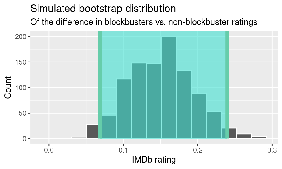
The resulting 95% confidence interval for the difference in means is (0.069, 0.239). We discuss the implications of the confidence interval and correlation coefficients in the following section.
2.3. Interpretation and conclusions
From the above data, we can see that the correlation between a film’s release year and IMDb rating is negligibly low—there appears to be virtually no association between these two variables, given that the correlation coefficient (r = 0.055) is near 0. We can also see that a film’s income has a weakly positive relationship with its rating—the correlation coefficient (r = 0.183) marks an improvement over that year vs. rating. As such, there appears to be a stronger relationship between a film’s income and rating than its release year and rating, albeit still quite weak.
When comparing the relationship between two numerical variables, correlation coefficients are the ideal statistical method, and the story told for the relationship (or lack thereof) between year and rating is quite clear. In essence, this result lends credence to the idea that overall film quality has not changed much over time—movie quality, at least as scored by IMDb, seems to have little to do with the year. It seems that the conventional wisdom that Hollywood is getting worse—from its increasing reliance on sequels to the shift to streaming services—does not quite hold water.
On the other hand, the fairly noticeable correlation between income and rating inspired us to find a confidence interval for the difference in the true mean ratings for blockbuster movies (films earning at least $100,000,000) versus non-blockbuster movies. After bootstrapping, we are 95% confident that the true mean rating for blockbusters is 0.069 to 0.239 higher than the true mean rating for non-blockbusters. Our interval does not include any negative numbers, which means that we are extremely confident that the true difference in mean ratings between blockbusters and non-blockbusters is positive—the average blockbuster will likely earn a better rating than a non-blockbuster. Going into this analysis, we believed it was possible that blockbusters would earn less than non-blockbusters made with a specific audience in mind, but, in the end, blockbusters tend to have higher ratings.
Limitations
In terms of limitations, because this data is based on the way IMDb scores popularity, it may not necessarily reflect how other sites or how others may think of a movie in terms of ranking and popularity. Rather than aggregate critic scores, IMDb ratings are user-sourced, which leaves them vulnerable to review-bombing and other coordinated campaigns to manipulate scoring. Thus, the data could be biased. In addition, some of the data has columns that are missing. For example, not all certificates have correlated values (34 certificates are missing). Another possible limitation is that if we were to use categories regarding budget or income, there are certain movies that have a missing budget or income. Finally, the data for income and ratings seem to be quite low in 2020, presumably because of the pandemic—movies received lower income and more noise exists in the data because of the smaller sample size, so COVID-19 likely presents a confounding variable for our analysis, especially when mapping changes in income/ratings over time. Our modelling and analysis is rigorous and accurate, but their validity relies on the correctness of the underlying data. Although COVID-19 and other factors represent a blip in our dataset—and while these limitations should be noted—we are confident that our conclusions are significant, correct, and useful.
Acknowledgments
The data that we used was provided on Kaggle by a user with the username GEORGE SCUTELNICU. We would like to thank this user for their scraping and cleaning, and we would like to thank Pin-Sung Ku for his project mentorship and Dr. Soltoff for his teaching.