The data was quite clean and tidy when we received it, but it contained some attributes (columns) that we did not need for our planned data analysis. Thus, we removed a few unneeded columns, including the names of the many actors involved, since we only want to focus on the main couple and the age gap between them. We then created a new variable that contained the age gap of the main couple, and organized it in order of descending age gap. For movies that had the same age gap, we ordered them by descending release year. We also created the variable years_since_start, which depicts the number of years since 1935 that a movie was released, because 1935 is the earliest year represented in our dataset of movies. We can calculate time intervals and trends and build models based on the elapsed years, which can provide valuable insights into how the movie age gaps have evolved over time. By representing time as the number of years since the first year in the data, we normalize the dataset and create a standardized scale that can be useful for comparison purposes.
Other appendicies (as necessary)
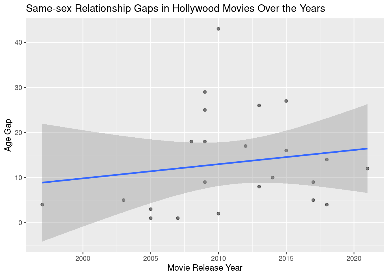
# Analysis 2: Same Sex vs. Heterosexual relationships over time# same-sex relationships in Hollywood movies over timehomo_movies_draft <- movies_clean |>filter(actor_1_gender == actor_2_gender)ggplot(data = homo_movies_draft, breaks=30, mapping =aes(x = release_year, y = age_gap)) +geom_point(alpha =0.5) +scale_color_viridis_d() +geom_smooth(method ="lm") +labs(title ="Same-sex Relationship Gaps in Hollywood Movies Over the Years",x ="Movie Release Year",y ="Age Gap" )
`geom_smooth()` using formula = 'y ~ x'
homo_age_gap_year_reg <-lm(age_gap ~ release_year, data = homo_movies_draft)tidy(homo_age_gap_year_reg)
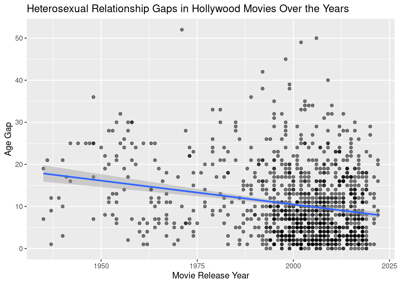
# heterosexual relationships in Hollywood movies over timehetero_movies_draft <- movies_clean |>filter(actor_1_gender != actor_2_gender)ggplot(data = hetero_movies_draft, breaks=30, mapping =aes(x = release_year, y = age_gap)) +geom_point(alpha =0.5) +scale_color_viridis_d() +geom_smooth(method ="lm") +labs(title ="Heterosexual Relationship Gaps in Hollywood Movies Over the Years",x ="Movie Release Year",y ="Age Gap" )
`geom_smooth()` using formula = 'y ~ x'
hetero_age_gap_year_reg <-lm(age_gap ~ release_year, data = hetero_movies_draft)tidy(hetero_age_gap_year_reg)
The first regression model above suggests that the age gap in movies with same-sex relationships have increased over the years. Although the relationship between the release year and age gap is weak because of a small sample size, there is still a loose suggestion that time affects the age gap in same-sex relationships because the linear regression line that is formed has a positive slope. The second regression model strongly suggests that there is a strong relationship between time and the age gap in heterosexual relationship gaps in Hollywood movies. It appears that as time passes, the age gap in heterosexual relationships in Hollywood movies decreases. This is evident in the fact that the points are closely located to one another in a dense cloud and the linear regression line has a negative slope.
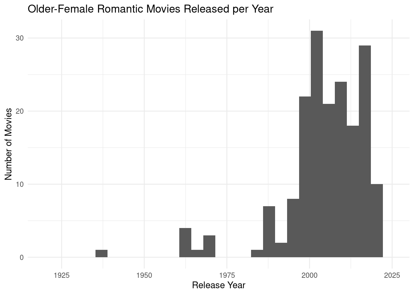
older_man_movies <- movies_clean |>filter(actor_1_gender != actor_2_gender) |>filter(actor_1_age > actor_2_age)older_woman_movies <- movies_clean |>filter(actor_1_gender != actor_2_gender) |>filter(actor_1_age < actor_2_age)# Dataset to reflect number of movies where the man is olderolder_man_movies_num <- older_man_movies |>group_by(release_year) |>count()# Dataset to reflect number of movies where the woman is olderolder_woman_movies_num <- older_woman_movies |>group_by(release_year) |>count()# Dataset to reflect number of movies with heterosexual coupleshetero_movies_num <- hetero_movies_draft |>group_by(release_year) |>count()# Dataset to reflect number of movies with homosexual coupleshomo_movies_num <- homo_movies_draft |>group_by(release_year) |>count()
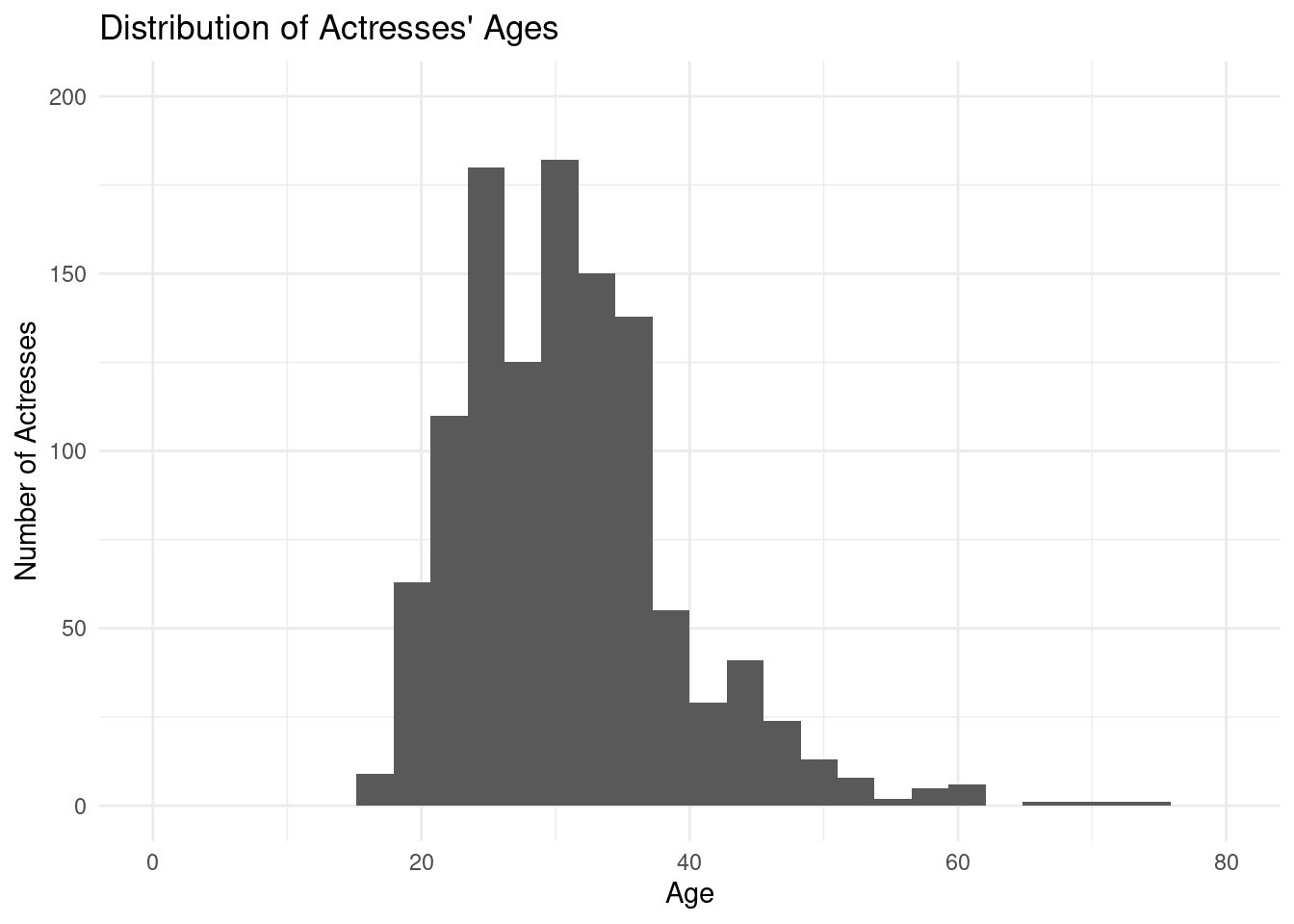
# Distribution of Actresses' Agesmovies_women <- movies_clean |>filter(actor_2_gender =="woman") |>mutate(actor_age = actor_2_age)ggplot(data = movies_women, mapping =aes(x = actor_age)) +scale_x_continuous(limits =c(0, 80)) +scale_y_continuous(limits =c(0, 200), n.breaks =5) +geom_histogram() +labs(title ="Distribution of Actresses' Ages",x ="Age",y ="Number of Actresses" ) +theme_minimal()
`stat_bin()` using `bins = 30`. Pick better value with `binwidth`.
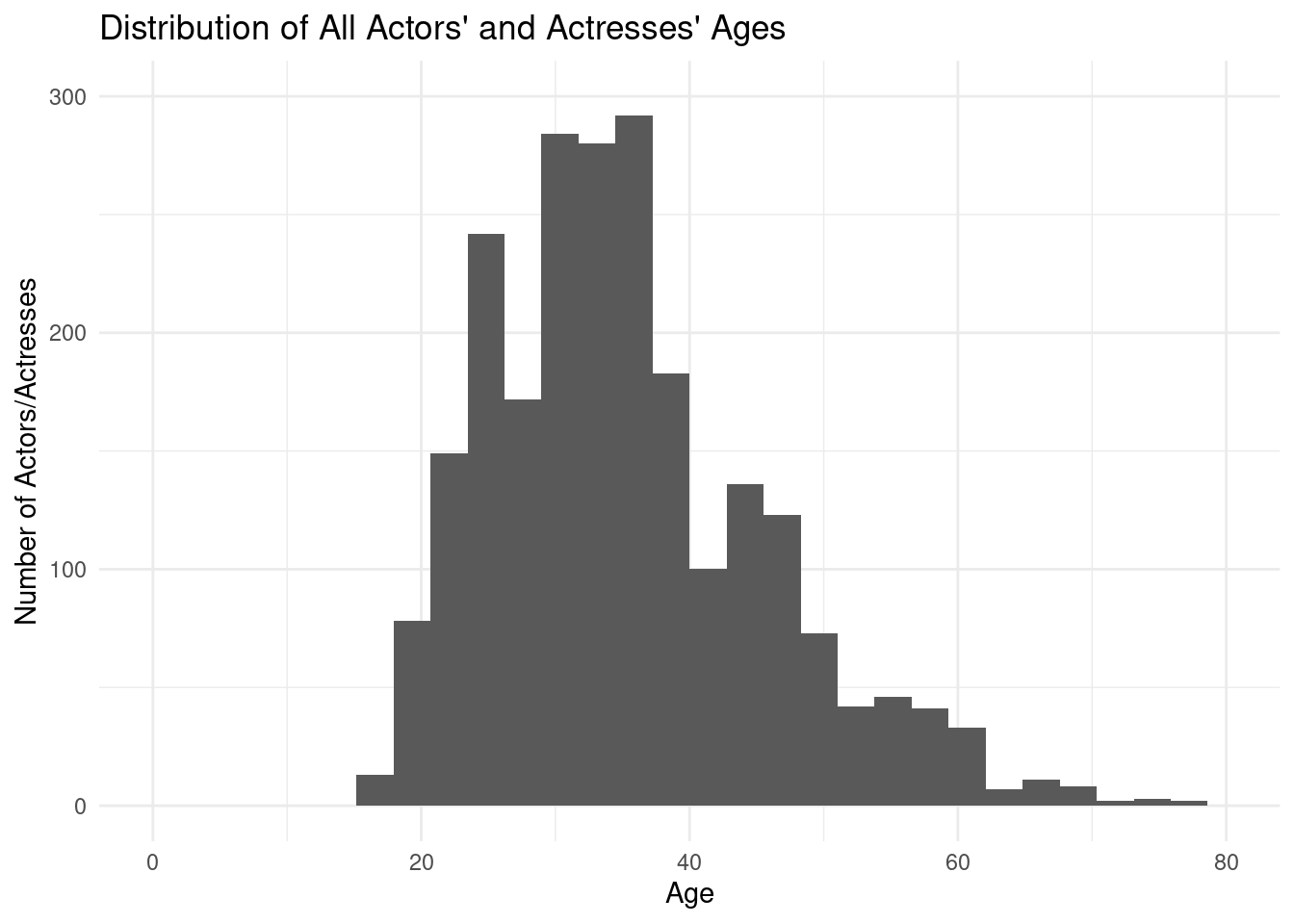
# Distribution of Ages of all Actors and Actresses in Datasetmovies_clean_all_ages <-bind_rows(movies_men, movies_women)all_ages <-c(movies_clean$actor_1_age, movies_clean$actor_2_age)ggplot(data =data.frame(x = all_ages), aes(x)) +scale_x_continuous(limits =c(0, 80)) +scale_y_continuous(limits =c(0, 300)) +geom_histogram() +labs(title ="Distribution of All Actors' and Actresses' Ages",x ="Age",y ="Number of Actors/Actresses" ) +theme_minimal()
`stat_bin()` using `bins = 30`. Pick better value with `binwidth`.
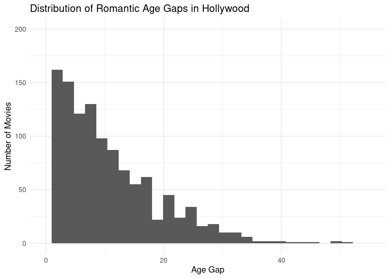
# Distribution of the romantic age gaps in our movie dataggplot(data = movies_clean, mapping =aes(x = age_gap)) +scale_x_continuous(limits =c(0, 55)) +scale_y_continuous(limits =c(0, 200), n.breaks =5) +geom_histogram() +labs(title ="Distribution of Romantic Age Gaps in Hollywood",x ="Age Gap",y ="Number of Movies" ) +theme_minimal()
`stat_bin()` using `bins = 30`. Pick better value with `binwidth`.
# Summary of movies by release yearsummary(movies_clean)
  movie_name         release_year    director         age_difference
 Length:1161        Min.   :1935   Length:1161        Min.   : 0.00
 Class :character   1st Qu.:1997   Class :character   1st Qu.: 4.00
 Mode  :character   Median :2004   Mode  :character   Median : 8.00
                    Mean   :2001                      Mean   :10.47
                    3rd Qu.:2012                      3rd Qu.:16.00
                    Max.   :2022                      Max.   :52.00
 actor_1_name       actor_1_gender     actor_1_birthdate   actor_1_age
 Length:1161        Length:1161        Length:1161        Min.   :17.00
 Class :character   Class :character   Class :character   1st Qu.:32.00
 Mode  :character   Mode  :character   Mode  :character   Median :38.00
                                                          Mean   :39.85
                                                          3rd Qu.:47.00
                                                          Max.   :81.00
 actor_2_name       actor_2_gender     actor_2_birthdate   actor_2_age
 Length:1161        Length:1161        Length:1161        Min.   :17.00
 Class :character   Class :character   Class :character   1st Qu.:25.00
 Mode  :character   Mode  :character   Mode  :character   Median :30.00
                                                          Mean   :31.06
                                                          3rd Qu.:35.00
                                                          Max.   :75.00
    age_gap      years_since_start
 Min.   : 0.00   Min.   : 0.00
 1st Qu.: 4.00   1st Qu.:62.00
 Median : 8.00   Median :69.00
 Mean   :10.47   Mean   :65.59
 3rd Qu.:16.00   3rd Qu.:77.00
 Max.   :52.00   Max.   :87.00
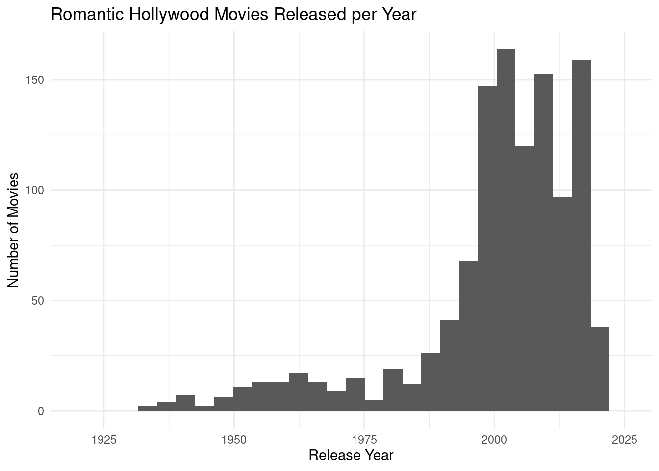
ggplot(data = movies_clean, mapping =aes(x = release_year)) +geom_histogram() +scale_x_continuous(limits =c(1920, 2025), n.breaks =5) +labs(title ="Romantic Hollywood Movies Released per Year",x ="Release Year",y ="Number of Movies" ) +theme_minimal()
`stat_bin()` using `bins = 30`. Pick better value with `binwidth`.
# Summary of older-man movies by release yearsummary(older_man_movies)
  movie_name         release_year    director         age_difference
 Length:926         Min.   :1935   Length:926         Min.   : 1.00
 Class :character   1st Qu.:1995   Class :character   1st Qu.: 5.00
 Mode  :character   Median :2003   Mode  :character   Median :10.00
                    Mean   :1999                      Mean   :11.76
                    3rd Qu.:2011                      3rd Qu.:17.00
                    Max.   :2022                      Max.   :50.00
 actor_1_name       actor_1_gender     actor_1_birthdate   actor_1_age
 Length:926         Length:926         Length:926         Min.   :19.00
 Class :character   Class :character   Class :character   1st Qu.:35.00
 Mode  :character   Mode  :character   Mode  :character   Median :40.00
                                                          Mean   :41.82
                                                          3rd Qu.:48.00
                                                          Max.   :79.00
 actor_2_name       actor_2_gender     actor_2_birthdate   actor_2_age
 Length:926         Length:926         Length:926         Min.   :17.00
 Class :character   Class :character   Class :character   1st Qu.:25.00
 Mode  :character   Mode  :character   Mode  :character   Median :29.00
                                                          Mean   :30.06
                                                          3rd Qu.:34.00
                                                          Max.   :68.00
    age_gap      years_since_start
 Min.   : 1.00   Min.   : 0.00
 1st Qu.: 5.00   1st Qu.:60.00
 Median :10.00   Median :68.00
 Mean   :11.76   Mean   :64.36
 3rd Qu.:17.00   3rd Qu.:76.00
 Max.   :50.00   Max.   :87.00
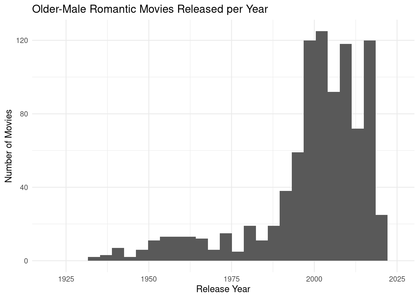
ggplot(data = older_man_movies, mapping =aes(x = release_year)) +geom_histogram() +scale_x_continuous(limits =c(1920, 2025), n.breaks =5) +labs(title ="Older-Male Romantic Movies Released per Year",x ="Release Year",y ="Number of Movies" ) +theme_minimal()
`stat_bin()` using `bins = 30`. Pick better value with `binwidth`.