Project title

Exploratory data analysis

Research question(s)

What is the relationship between average song hotness (popularity) and the year it was released?
Does song tempo influence song popularity?
Does song duration influence song popularity?
What is the relationship between artist familiarity and their song popularity?

Data collection and cleaning

Have an initial draft of your data cleaning appendix. Document every step that takes your raw data file(s) and turns it into the analysis-ready data set that you would submit with your final project. Include text narrative describing your data collection (downloading, scraping, surveys, etc) and any additional data curation/cleaning (merging data frames, filtering, transformations of variables, etc). Include code for data curation/cleaning, but not collection.

library(tidyverse)

── Attaching packages ─────────────────────────────────────── tidyverse 1.3.2 ──
✔ ggplot2 3.4.2     ✔ purrr   1.0.0
✔ tibble  3.2.1     ✔ dplyr   1.1.2
✔ tidyr   1.2.1     ✔ stringr 1.5.0
✔ readr   2.1.3     ✔ forcats 0.5.2
── Conflicts ────────────────────────────────────────── tidyverse_conflicts() ──
✖ dplyr::filter() masks stats::filter()
✖ dplyr::lag()    masks stats::lag()

music <- read_csv("data/music.csv")

Rows: 10000 Columns: 35
── Column specification ────────────────────────────────────────────────────────
Delimiter: ","
chr  (4): artist.id, artist.name, artist.terms, song.id
dbl (31): artist.familiarity, artist.hotttnesss, artist.latitude, artist.loc...

ℹ Use `spec()` to retrieve the full column specification for this data.
ℹ Specify the column types or set `show_col_types = FALSE` to quiet this message.

tidy_music <- music |>
  # selecting the variables we are using out of the original dataset
  select(artist.name, artist.id, artist.terms, 
         artist.familiarity, artist.hotttnesss, song.hotttnesss, 
         song.id, song.year, song.tempo, song.duration) |>
  filter(
    # only include the observations that have a recorded song year
    song.year != 0, 
    
    # and observations where hotness is in the scale the data was measured in.
    song.hotttnesss > 0,
      artist.familiarity != 0,
    artist.hotttnesss != 0,
    song.tempo != 0
  ) 


  

tidy_music

# A tibble: 2,693 × 10
   artist.name       artist.id artist.terms artist.familiarity artist.hotttnesss
   <chr>             <chr>     <chr>                     <dbl>             <dbl>
 1 Gob               ARXR32B1… pop punk                  0.651             0.402
 2 Planet P Project  AR8ZCNI1… new wave                  0.427             0.332
 3 Blue Rodeo        ARD842G1… country rock              0.636             0.448
 4 Tesla             ARYKCQI1… hard rock                 0.707             0.513
 5 The Dillinger Es… ARMAC4T1… math-core                 0.840             0.542
 6 SUE THOMPSON      AR47JEX1… pop rock                  0.435             0.306
 7 Terry Callier     ARB29H41… soul jazz                 0.707             0.416
 8 The Shangri-Las   ARAJPHH1… doo-wop                   0.641             0.418
 9 Scarlet's Remains ARLGWFM1… gothic metal              0.528             0.393
10 The Suicide Mach… ARWYVP51… ska punk                  0.669             0.468
# ℹ 2,683 more rows
# ℹ 5 more variables: song.hotttnesss <dbl>, song.id <chr>, song.year <dbl>,
#   song.tempo <dbl>, song.duration <dbl>

#looking at the artist terms to see the frequency of use for each one
tidy_music |>
  group_by(artist.terms)|>
  count()

# A tibble: 296 × 2
# Groups:   artist.terms [296]
   artist.terms            n
   <chr>               <int>
 1 acid jazz               1
 2 afrobeat                2
 3 all-female              1
 4 alternative country     1
 5 alternative dance      19
 6 alternative hip hop     4
 7 alternative metal      40
 8 alternative rap         1
 9 alternative rock       14
10 arabesque               1
# ℹ 286 more rows

#organizing each song into major genres pop, rap/hip hop/rock/electronic/country/jazz/soul/other
#using the table above to include subgenres into the major genres.
#looking through every artist term and to pick out the term, organizing by whichever major genre appears first
tidy_music <- tidy_music|>
  mutate(
    genre = if_else(
      grepl("pop", artist.terms), "Pop",
      if_else(
        grepl("rap|hip hop|grime|hop", artist.terms), "Rap/Hip hop",
        if_else(
          grepl("rock|metal|punk|death core|grunge|hardcore", artist.terms), "Rock",
          if_else(
            grepl("electronic|techno|tech", artist.terms), "Electronic",
            if_else(
              grepl("country", artist.terms), "Country",
              if_else(
                grepl("jazz|blues", artist.terms), "Jazz",
                if_else(
                  grepl("soul", artist.terms), "Soul", "Other"
                )
              )
            )
          )
        )
      )
    )
  )
tidy_music

# A tibble: 2,693 × 11
   artist.name       artist.id artist.terms artist.familiarity artist.hotttnesss
   <chr>             <chr>     <chr>                     <dbl>             <dbl>
 1 Gob               ARXR32B1… pop punk                  0.651             0.402
 2 Planet P Project  AR8ZCNI1… new wave                  0.427             0.332
 3 Blue Rodeo        ARD842G1… country rock              0.636             0.448
 4 Tesla             ARYKCQI1… hard rock                 0.707             0.513
 5 The Dillinger Es… ARMAC4T1… math-core                 0.840             0.542
 6 SUE THOMPSON      AR47JEX1… pop rock                  0.435             0.306
 7 Terry Callier     ARB29H41… soul jazz                 0.707             0.416
 8 The Shangri-Las   ARAJPHH1… doo-wop                   0.641             0.418
 9 Scarlet's Remains ARLGWFM1… gothic metal              0.528             0.393
10 The Suicide Mach… ARWYVP51… ska punk                  0.669             0.468
# ℹ 2,683 more rows
# ℹ 6 more variables: song.hotttnesss <dbl>, song.id <chr>, song.year <dbl>,
#   song.tempo <dbl>, song.duration <dbl>, genre <chr>

write.csv(tidy_music, "data/tidy_music.csv")

Data description

Our data is from the Million Song Dataset, which used a company called the Echo Nest to derive data points about one million popular contemporary songs. The Million Song Dataset is a collaboration between the Echo Nest. The data was collected to encourage research on algorithms that scale to commercial sizes and to provide a reference datasets for evaluating research. The data contains standard information about the songs such as artist name, title, identification, song duration and year released that we can use to help with the data to answer our research question is the popularity of the song, the popularity of the artist, the terms used to describe the artists, and song tempo.

Data limitations

The artists’ terms are not always associated with a specific genre or common name for a genre; therefore, it is difficult to identify which genre every song in our dataset might belong in.

Exploratory data analysis

Perform an (initial) exploratory data analysis.

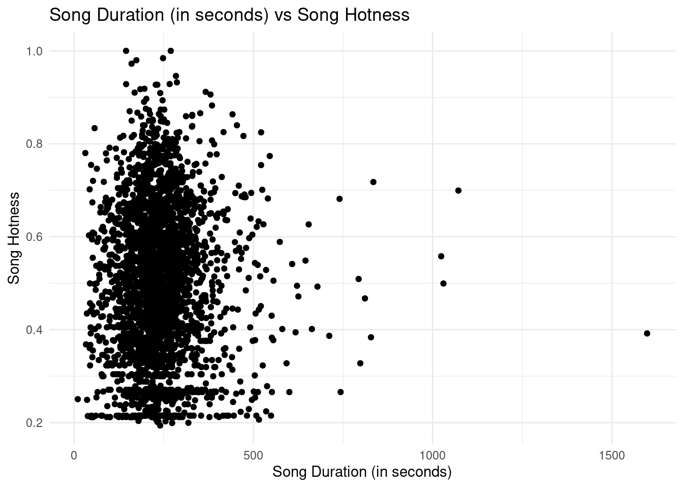
ggplot(data = tidy_music, mapping = aes(x = song.duration, y = song.hotttnesss)) + 
  geom_point() + 
  labs(
    x = "Song Duration (in seconds)",
    y = "Song Hotness",
    title = "Song Duration (in seconds) vs Song Hotness"
  ) + 
  theme_minimal()

The scatter plot above explores the relationship between song duration (in seconds) and song hotness. For the most part, song duration, the length of a song does not seem to have an effect on how popular the song is later because most songs are relatively the same length. The hottest songs are usually 250 seconds long.

library(tidymodels)

── Attaching packages ────────────────────────────────────── tidymodels 1.0.0 ──

✔ broom        1.0.2     ✔ rsample      1.1.1
✔ dials        1.1.0     ✔ tune         1.1.1
✔ infer        1.0.4     ✔ workflows    1.1.2
✔ modeldata    1.0.1     ✔ workflowsets 1.0.0
✔ parsnip      1.0.3     ✔ yardstick    1.1.0
✔ recipes      1.0.6

── Conflicts ───────────────────────────────────────── tidymodels_conflicts() ──
✖ scales::discard() masks purrr::discard()
✖ dplyr::filter()   masks stats::filter()
✖ recipes::fixed()  masks stringr::fixed()
✖ dplyr::lag()      masks stats::lag()
✖ yardstick::spec() masks readr::spec()
✖ recipes::step()   masks stats::step()
• Search for functions across packages at https://www.tidymodels.org/find/

tempo_pop_fit <- linear_reg() |>
  fit(song.hotttnesss ~ song.tempo, data = tidy_music)

tidy(tempo_pop_fit)

# A tibble: 2 × 5
  term        estimate std.error statistic   p.value
  <chr>          <dbl>     <dbl>     <dbl>     <dbl>
1 (Intercept) 0.467    0.0119        39.3  5.22e-267
2 song.tempo  0.000288 0.0000907      3.17 1.52e-  3

ggplot(tidy_music, aes(x = song.tempo, y = song.hotttnesss)) +
  geom_point() +
  geom_smooth(method = "lm")

`geom_smooth()` using formula = 'y ~ x'

\[ \widehat{song~hotness} = 0.40 + 0.00043 \times song~tempo \]

If a song has a tempo of 0 BPM, the hotness is expected to be 0.40, on average. For each increase in song tempo, the song popularity is expected to be higher by 0.00043, on average. In this scatter plot visualization, a positive association can be seen between song tempo and song popularity when looking at the linear regression line.

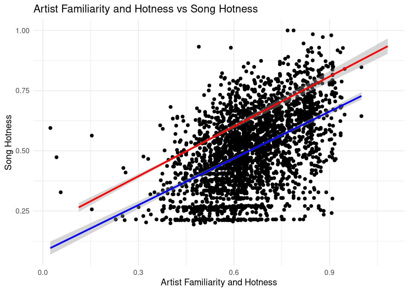
ggplot(data = tidy_music, mapping = aes(x = artist.familiarity, y = song.hotttnesss)) + 
  geom_point() + 
  geom_smooth(method = "lm") +
  labs(
    x = "Artist Familiarity",
    y = "Song Hotness",
    title = "Artist Familiarity vs Song Hotness"
  ) + 
  theme_minimal()

`geom_smooth()` using formula = 'y ~ x'

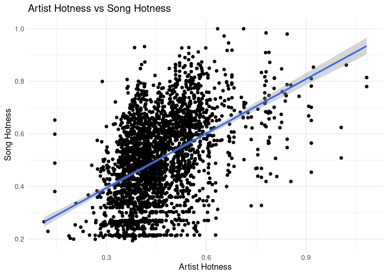
ggplot(data = tidy_music, mapping = aes(x = artist.hotttnesss, y = song.hotttnesss)) + 
  geom_point() + 
  geom_smooth(method = "lm") +
  labs(
    x = "Artist Hotness",
    y = "Song Hotness",
    title = "Artist Hotness vs Song Hotness"
  ) + 
  theme_minimal()

`geom_smooth()` using formula = 'y ~ x'

artist_song_hotness <- linear_reg() |>
  fit(song.hotttnesss ~ artist.familiarity, data = tidy_music)

artist_song_fam <- linear_reg() |>
  fit(song.hotttnesss ~ artist.hotttnesss, data = tidy_music)

tidy(artist_song_hotness)

# A tibble: 2 × 5
  term               estimate std.error statistic   p.value
  <chr>                 <dbl>     <dbl>     <dbl>     <dbl>
1 (Intercept)          0.0810    0.0144      5.63 1.99e-  8
2 artist.familiarity   0.647     0.0216     29.9  9.16e-170

tidy(artist_song_fam)

# A tibble: 2 × 5
  term              estimate std.error statistic   p.value
  <chr>                <dbl>     <dbl>     <dbl>     <dbl>
1 (Intercept)          0.187    0.0121      15.5 6.09e- 52
2 artist.hotttnesss    0.690    0.0257      26.8 1.54e-140

glance(artist_song_hotness)

# A tibble: 1 × 12
  r.squared adj.r.squared sigma statistic   p.value    df logLik    AIC    BIC
      <dbl>         <dbl> <dbl>     <dbl>     <dbl> <dbl>  <dbl>  <dbl>  <dbl>
1     0.249         0.249 0.142      893. 9.16e-170     1  1434. -2861. -2844.
# ℹ 3 more variables: deviance <dbl>, df.residual <int>, nobs <int>

glance(artist_song_fam)

# A tibble: 1 × 12
  r.squared adj.r.squared sigma statistic   p.value    df logLik    AIC    BIC
      <dbl>         <dbl> <dbl>     <dbl>     <dbl> <dbl>  <dbl>  <dbl>  <dbl>
1     0.211         0.211 0.146      719. 1.54e-140     1  1366. -2727. -2709.
# ℹ 3 more variables: deviance <dbl>, df.residual <int>, nobs <int>

\[ \widehat{song~hotness} = -0.12 + 0.88 \times artist~familiarity \]

\[ \widehat{song~hotness} = 0.02 + 0.94 \times artist~hotness \]

A positive correlation can be seen when plotting “song hotness” against “artist hotness” and “artist popularity”. That is, the hotter or more popular the artist is, the hotter the song is expected to be. The intercepts of the two equations mean that artist with no familiarity or hotness will have their song expected to be not hot at all. The first slope mean that with a point increase in artist familiarity, song hotness is expected to increase by .88 points. Similarly, with a point increase in artist hotness, song hotness is expected to increase by .94 points. Also, the models explain more than 20% of the variability.

library(tidyverse)
tidy_music <- read_csv("data/tidy_music.csv")

New names:
Rows: 2693 Columns: 12
── Column specification
──────────────────────────────────────────────────────── Delimiter: "," chr
(5): artist.name, artist.id, artist.terms, song.id, genre dbl (7): ...1,
artist.familiarity, artist.hotttnesss, song.hotttnesss, song....
ℹ Use `spec()` to retrieve the full column specification for this data. ℹ
Specify the column types or set `show_col_types = FALSE` to quiet this message.
• `` -> `...1`

library(tidymodels)

tempo_pop_fit <- linear_reg() |>
  fit(song.hotttnesss ~ song.tempo*genre, data = tidy_music)

tidy(tempo_pop_fit)

# A tibble: 16 × 5
   term                         estimate std.error statistic      p.value
   <chr>                           <dbl>     <dbl>     <dbl>        <dbl>
 1 (Intercept)                  0.560     0.103        5.43  0.0000000600
 2 song.tempo                  -0.000528  0.000782    -0.675 0.500       
 3 genreElectronic             -0.0871    0.141       -0.617 0.537       
 4 genreJazz                   -0.173     0.110       -1.58  0.114       
 5 genreOther                  -0.145     0.105       -1.38  0.169       
 6 genrePop                    -0.0889    0.110       -0.812 0.417       
 7 genreRap/Hip hop             0.0246    0.108        0.227 0.820       
 8 genreRock                   -0.0534    0.105       -0.510 0.610       
 9 genreSoul                   -0.138     0.143       -0.962 0.336       
10 song.tempo:genreElectronic   0.000877  0.00108      0.814 0.416       
11 song.tempo:genreJazz         0.000755  0.000838     0.901 0.368       
12 song.tempo:genreOther        0.000786  0.000799     0.984 0.325       
13 song.tempo:genrePop          0.00103   0.000833     1.24  0.214       
14 song.tempo:genreRap/Hip hop  0.000124  0.000824     0.151 0.880       
15 song.tempo:genreRock         0.000800  0.000795     1.01  0.314       
16 song.tempo:genreSoul         0.00129   0.00116      1.12  0.264

ggplot(tidy_music, aes(x = song.tempo, y = song.hotttnesss, color = genre)) +
  geom_point(alpha = 0.1) +
  geom_smooth(method = "lm", se = FALSE) +
  facet_wrap(facets = vars(genre), nrow = 2) +
  scale_color_viridis_d(option = "H") +
  theme_minimal()

`geom_smooth()` using formula = 'y ~ x'

artist_song_model <- lm(song.hotttnesss ~ artist.familiarity + artist.hotttnesss, data = tidy_music)
ggplot(data = tidy_music, mapping = aes(x = artist.familiarity, y = song.hotttnesss)) + 
  geom_point() + 
  geom_smooth(method = "lm", aes(x = artist.familiarity, y = song.hotttnesss), color = "blue") +
  geom_smooth(method = "lm", aes(x = artist.hotttnesss, y = song.hotttnesss), color = "red") +
  labs(
    x = "Artist Familiarity and Hotness",
    y = "Song Hotness",
    title = "Artist Familiarity and Hotness vs Song Hotness"
  ) + 
  theme_minimal()

`geom_smooth()` using formula = 'y ~ x'
`geom_smooth()` using formula = 'y ~ x'

tidy(artist_song_model)

# A tibble: 3 × 5
  term               estimate std.error statistic  p.value
  <chr>                 <dbl>     <dbl>     <dbl>    <dbl>
1 (Intercept)          0.0764    0.0143      5.35 9.72e- 8
2 artist.familiarity   0.468     0.0345     13.6  1.23e-40
3 artist.hotttnesss    0.266     0.0400      6.65 3.63e-11

glance(artist_song_model)

# A tibble: 1 × 12
  r.squared adj.r.squared sigma statistic   p.value    df logLik    AIC    BIC
      <dbl>         <dbl> <dbl>     <dbl>     <dbl> <dbl>  <dbl>  <dbl>  <dbl>
1     0.261         0.261 0.141      476. 1.05e-177     2  1456. -2903. -2880.
# ℹ 3 more variables: deviance <dbl>, df.residual <int>, nobs <int>

Questions for reviewers

List specific questions for your peer reviewers and project mentor to answer in giving you feedback on this phase.

Do we have strong research questions and enough data to complete this project?
Looking at our data, what kind of visualizations do you think we should use?