── Attaching packages ─────────────────────────────────────── tidyverse 1.3.2 ──
✔ ggplot2 3.4.2     ✔ purrr   1.0.0
✔ tibble  3.2.1     ✔ dplyr   1.1.2
✔ tidyr   1.2.1     ✔ stringr 1.5.0
✔ readr   2.1.3     ✔ forcats 0.5.2
── Conflicts ────────────────────────────────────────── tidyverse_conflicts() ──
✖ dplyr::filter() masks stats::filter()
✖ dplyr::lag()    masks stats::lag()
── Attaching packages ────────────────────────────────────── tidymodels 1.0.0 ──

✔ broom        1.0.2     ✔ rsample      1.1.1
✔ dials        1.1.0     ✔ tune         1.1.1
✔ infer        1.0.4     ✔ workflows    1.1.2
✔ modeldata    1.0.1     ✔ workflowsets 1.0.0
✔ parsnip      1.0.3     ✔ yardstick    1.1.0
✔ recipes      1.0.6

── Conflicts ───────────────────────────────────────── tidymodels_conflicts() ──
✖ scales::discard() masks purrr::discard()
✖ dplyr::filter()   masks stats::filter()
✖ recipes::fixed()  masks stringr::fixed()
✖ dplyr::lag()      masks stats::lag()
✖ yardstick::spec() masks readr::spec()
✖ recipes::step()   masks stats::step()
• Use tidymodels_prefer() to resolve common conflicts.

Loading required package: airports

Loading required package: cherryblossom

Loading required package: usdata


Attaching package: 'openintro'


The following object is masked from 'package:modeldata':

amesWhat Makes a Song Hottt!
Report
Introduction
All of us have a passion for music; we love to listen to songs on our walks to class, studying, or hanging out with friends. We wonder what draws us or others to certain types of songs or genres of music. What truly makes us like a song? To find answers to our questions, we found the Million Song Data set which contains information on one million contemporary songs. We would like to answer this research question, if the duration of a song, the tempo of a song, artists familiarity, and artist popularity influence the popularity of a song?
Using the Million Song Data set, we found that there is a positive relationship between song tempo and song hotness. For each unit increase in song tempo, the song hotness is expected to be higher. We also discovered certain variables that have minimal effect on song’s popularity: song duration and song hotness. Most importantly, we found a strong, positive correlation between the effect of artist hotness and artist familiarity on song popularity, leading us to believe that artist hotness and artist familiarity have a great effect on the popularity of a song.
We have a particular interest in this data because we think it could be connected to ways real up in coming artist could learn about the music industry. It also helps us as avid music listeners understand why some songs become popular and why others do not. It helps us understand why each of us know different artist and songs and helps us connect with music.
Data description
The observations (rows) are songs and the attributes (columns) are artist.id, artist.latitude, artist.longitude, artist.terms, song.hotttnesss, song.id, song.year, song.tempo. The data also includes standard information about the songs such as artist name, title, identification, song duration and year released.
Million Song Data set is a freely-available collection of audio features and metadata for a million contemporary popular music tracks. Our data is from the Million Song Data set, which used Echo Nest, the parent company of Spotify to derive data points about one million popular contemporary songs. The Million Song Data set started out as a collaboration project between the The Echo Nest and LabROSA, a laboratory working towards intelligent machine listening. The purpose of this data set is to encourage research on algorithms that scale to commercial sizes, provide a reference data set for evaluating research, service as a shortcut alternative to creating a large data set with APIs (e.g. The Echo Nest’s), and help new researchers get started in the MIR field.
Since Echo Nest is the parent company of Spotify, it is possible that a great portion of our data solely derives from one streaming platform, Spotify. This makes us question if other streaming platforms such as Apple Music, Pandora, or Sound Cloud are taken into consideration when we come to conclusions using this data.
The prepossessing that was done was to filter out the dataset was that we took out the 0 values, n/a values and the -1 values (not on the scale that it is measured by) and that left us with around 2693 songs to work with in out data.
It is likely that the users streaming music on certain platforms were aware of some potential data collection as it would have been mentioned in the terms and conditions. The data was collected to research, and it is not clear whether the individuals streaming the music were aware of the specific research question we are trying to answer with this data.
Data analysis
New names:
Rows: 2693 Columns: 12
── Column specification
──────────────────────────────────────────────────────── Delimiter: "," chr
(5): artist.name, artist.id, artist.terms, song.id, genre dbl (7): ...1,
artist.familiarity, artist.hotttnesss, song.hotttnesss, song....
ℹ Use `spec()` to retrieve the full column specification for this data. ℹ
Specify the column types or set `show_col_types = FALSE` to quiet this message.
• `` -> `...1`
# A tibble: 1 × 9
s.hotness_mean s.hotness_sd s.duration_mean s.duration_sd s.duration_median
<dbl> <dbl> <dbl> <dbl> <dbl>
1 0.503 0.164 240. 99.6 230.
# ℹ 4 more variables: s.tempo_mean <dbl>, s.tempo_sd <dbl>,
# a.hotness_mean <dbl>, a.hotness_sd <dbl>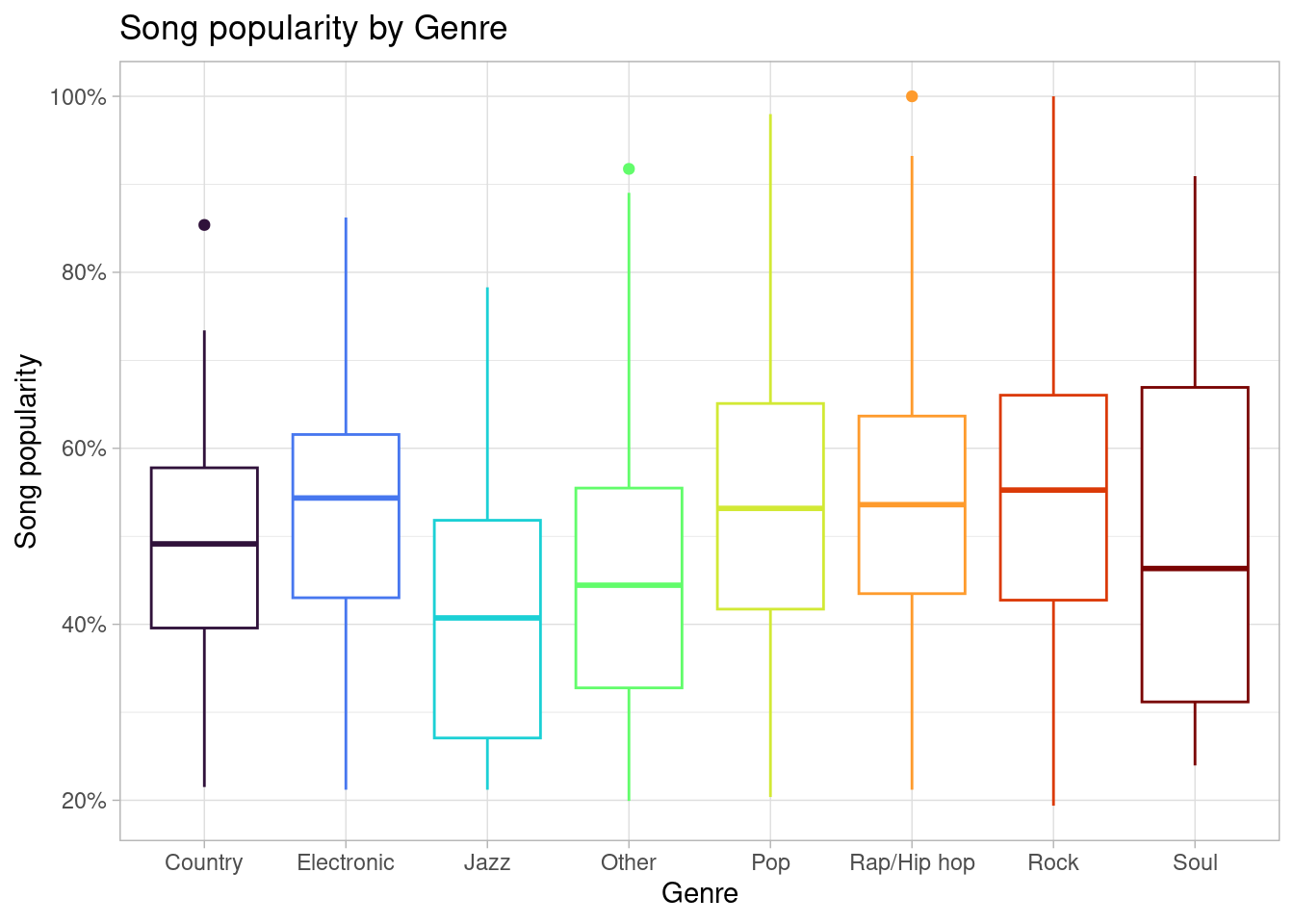
`geom_smooth()` using method = 'gam' and formula = 'y ~ s(x, bs = "cs")'
Song tempo and song hotness (popularity) seem to have a weak positive correlation.
`geom_smooth()` using formula = 'y ~ x'
Song duration and song hotness seem to have a small negative parabolic correlation with the peak being at around 229.80 seconds. There are also some pretty extreme outliers that skew the data.
# A tibble: 4 × 5
  term                         estimate   std.error statistic  p.value
  <chr>                           <dbl>       <dbl>     <dbl>    <dbl>
1 (Intercept)               0.447       0.0281         15.9   2.12e-54
2 song.tempo                0.000442    0.000223        1.98  4.76e- 2
3 song.duration             0.0000845   0.000108        0.780 4.35e- 1
4 song.tempo:song.duration -0.000000656 0.000000872    -0.752 4.52e- 1
# A tibble: 1 × 12
r.squared adj.r.squared sigma statistic p.value df logLik AIC BIC
<dbl> <dbl> <dbl> <dbl> <dbl> <dbl> <dbl> <dbl> <dbl>
1 0.00396 0.00285 0.164 3.56 0.0137 3 1053. -2096. -2066.
# ℹ 3 more variables: deviance <dbl>, df.residual <int>, nobs <int>\[ \begin{split} song~hotness = 0.000515 \times song~tempo + 0.000130 \times song~duration \\ - 0.000001 \times song~tempo \times song~duration + 0.0437 \end{split} \]
Intercept: when song tempo and song duration is 0, we expect song hotness to be 4.37%, on average.
Slopes: Keeping song duration constant, when song tempo increases by 1 BPM, song hotness is expected to increase by 0.0515% - 0.0001% * song duration, on average. Keeping song tempo constant, when song duration increases by 1 second, song hotness is expected to increase by 0.0130% - 0.0001% * song tempo, on average.
`geom_smooth()` using formula = 'y ~ x'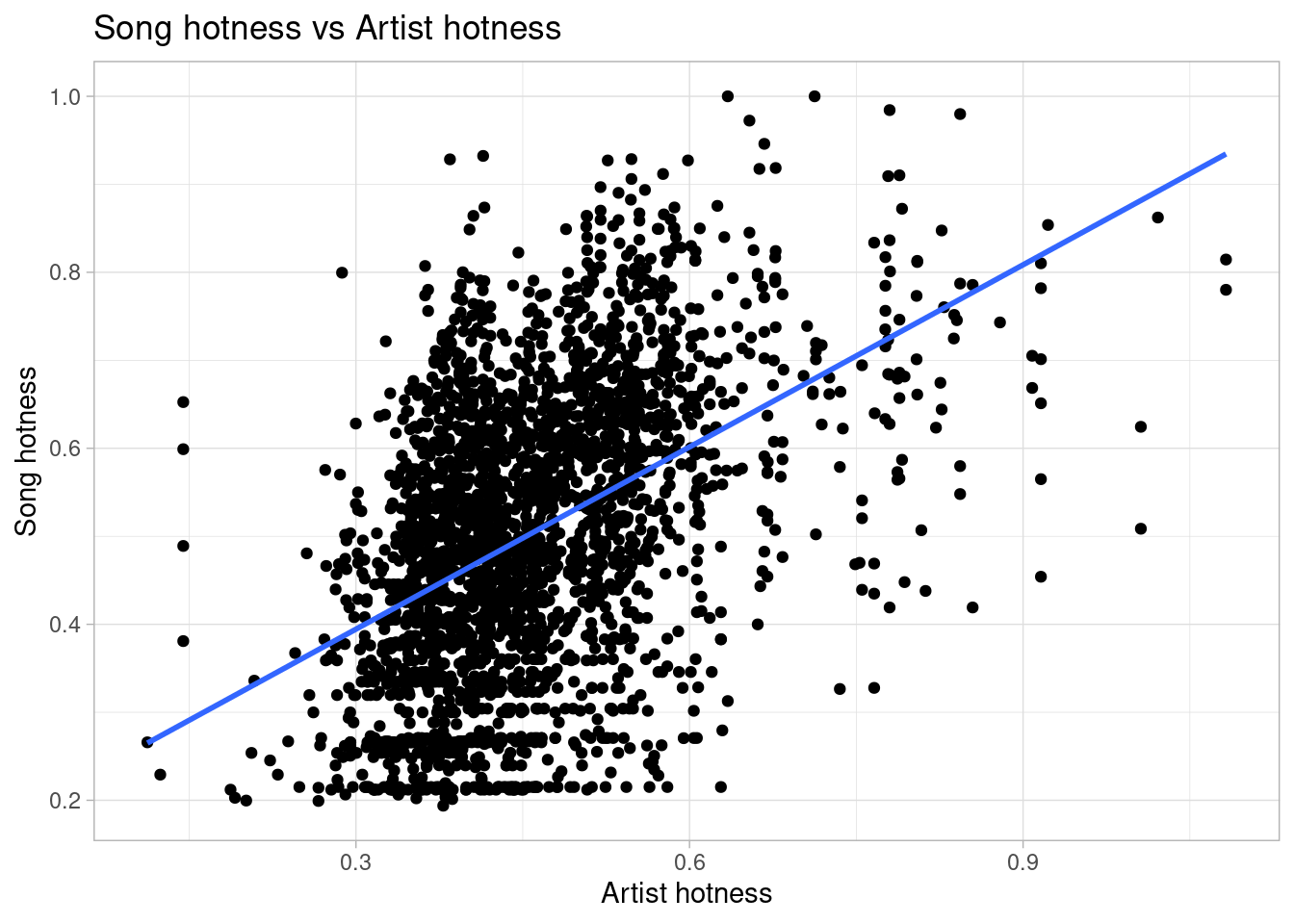
Artist popularity has a positive correlation with song popularity.
`geom_smooth()` using formula = 'y ~ x'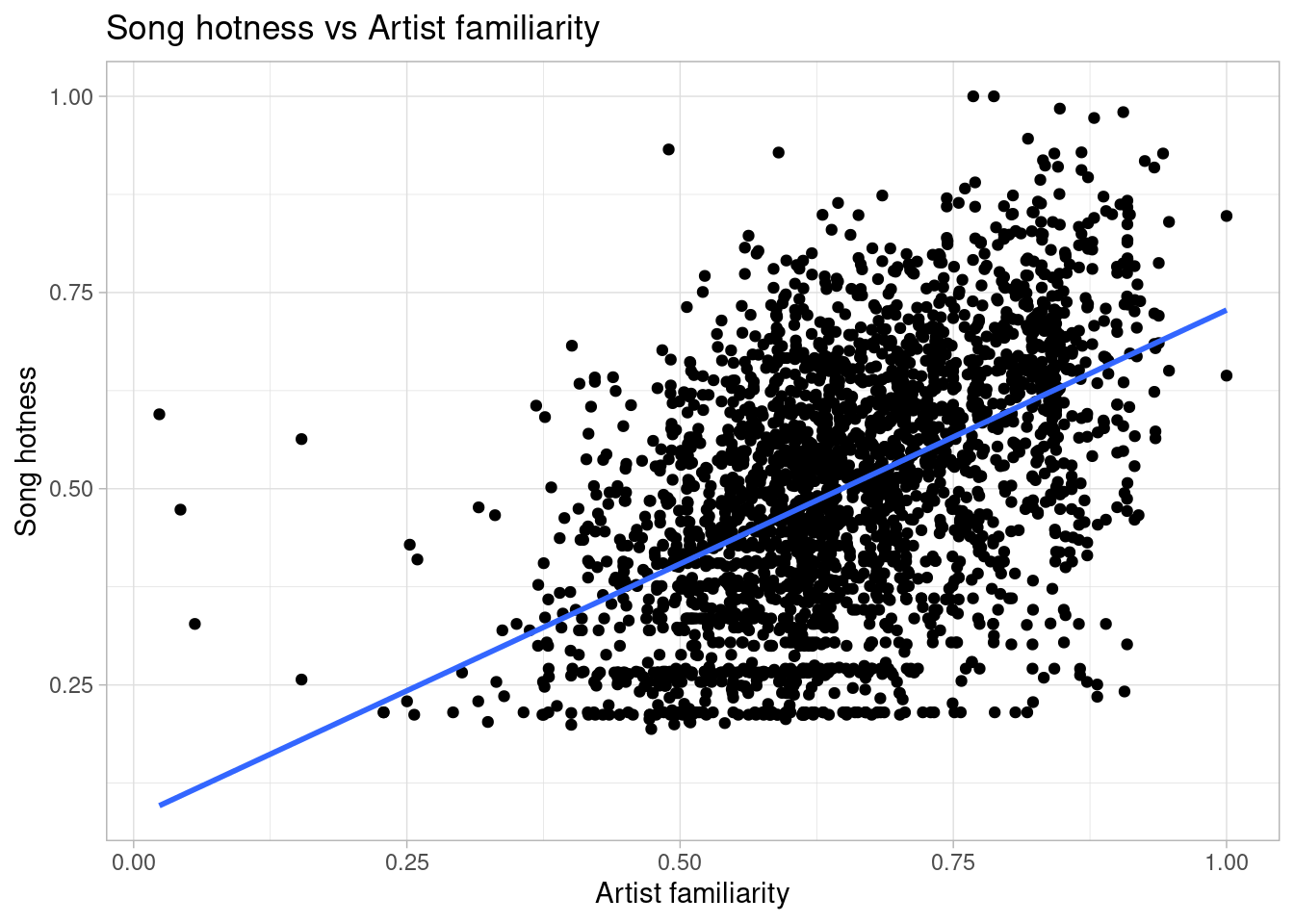
The familiarity of the artist also has a positive correlation with song popularity
# A tibble: 4 × 5
  term                                 estimate std.error statistic  p.value
  <chr>                                   <dbl>     <dbl>     <dbl>    <dbl>
1 (Intercept)                           0.00690    0.0565     0.122 9.03e- 1
2 artist.hotttnesss                     0.440      0.143      3.08  2.12e- 3
3 artist.familiarity                    0.559      0.0799     7.00  3.27e-12
4 artist.hotttnesss:artist.familiarity -0.227      0.179     -1.27  2.04e- 1
# A tibble: 1 × 12
r.squared adj.r.squared sigma statistic p.value df logLik AIC BIC
<dbl> <dbl> <dbl> <dbl> <dbl> <dbl> <dbl> <dbl> <dbl>
1 0.262 0.261 0.141 318. 1.16e-176 3 1456. -2903. -2873.
# ℹ 3 more variables: deviance <dbl>, df.residual <int>, nobs <int>Individually the artist hotness and familiarity have a greater effect on song hotness than both of them combined
\[ \begin{split}song~hotness = 0.00630 + 0.442\times artist~hotttnesss + 0.560 \times artist~familiarity \\-0.229\times artist~hotttnesss \times artist~familiarity \end{split} \]
Intercepts: When artist hotness and artist familiarity are 0 the song hotness on average is -0.630%.
Slopes: Holding artist familiarity constant, when artist hotness increases by 1 percentage, song hotness will increase by 44.2% - 22.9% * artist hotness, on average. Holding artist hotness constant, when artist familiarity increases by 1 percentage, song hotness increases by 56.0% - 22.9% * artist familiarity.
Evaluation of significance
Analysis 1:
The adjusted R2 of 0.0028 for the linear model using song tempo and song duration signifies that around 0.28% of the variability in song popularity is explained by the model. Hence, song tempo and song duration are not great predictors for song popularity.
We want to further examine the relationship between song tempo and song popularity. Therefore, we conduct a hypothesis test to check if there is a significant difference between the proportion of songs with hotness (popularity) greater than 0.8 inside and outside the tempo of 100-140 bpm. We chose this range because an average song will have a tempo in between 100-140bpm, and we define songs with popularity score greater than 0.8 to be “popular” songs.
1) Null Hypothesis:
\[ p_{100-140} - p_{outside} = 0 \]
The difference in proportion of 100-140 bpm songs with hotness greater than 0.8 and the proportion of bpm outside that range is equal to zero.
2) Alternative Hypothesis:
\[ p_{100-140} - p_{outside} \ne 0 \]
The difference in proportion of 100-140 bpm songs with hotness greater than 0.8 and the proportion of bpm outside that range is not equal to zero.
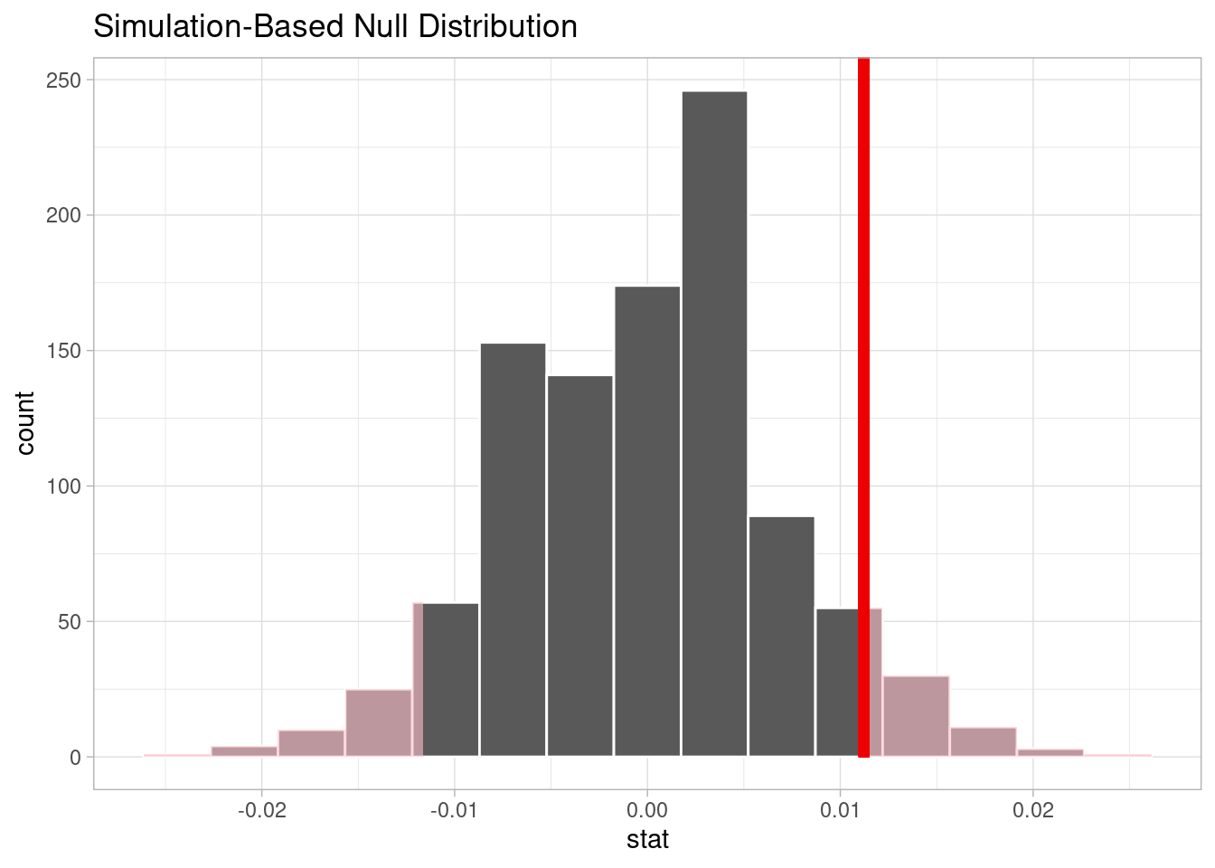
# A tibble: 1 × 1
  p_value
    <dbl>
1   0.132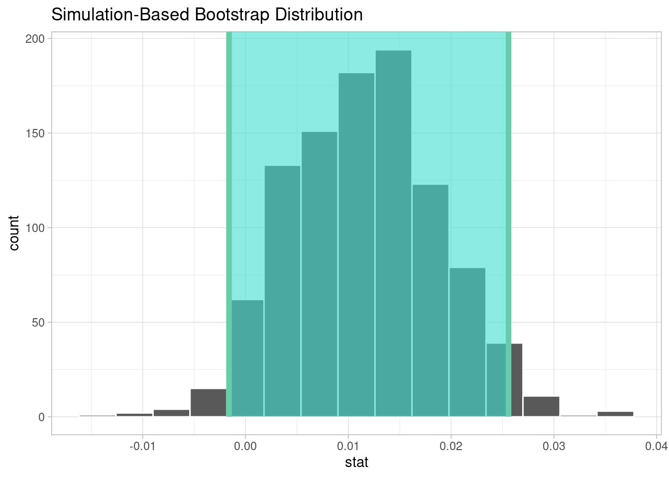
# A tibble: 1 × 2
  lower_ci upper_ci
     <dbl>    <dbl>
1 -0.00160   0.0256
Since the p-value is 0.132 and greater than the significance value of 0.05, we fail to reject the null hypothesis. Therefore, the data does not provide convincing evidence that the proportion of 100-140 bpm songs with hotness greater than 0.8 is different from the proportion of outside-range bpm songs with hotness greater than 0.8.
With this result, we can further conclude that a song’s success is not limited by tempo choice. Since no particular tempo range has a higher popular rate, artists can be free with their creativity and create songs with tempo they desire without worrying if that may affect the popularity of their songs.
We believe that this can be seen in why slow songs and faster pace songs both seem to be popular. Whether that is listening to the radio, streaming, or looking at songs that win awards, we see that both slow and fast-tempo songs are popular. Tempo differences should not deter an artist to create one or the other.
Analysis 2:
Next, we want to examine if there is a relationship between artist familiarity and song popularity. Therefore, we conduct a hypothesis test to check if there is a significant difference between the proportion of “hot” songs between “familiar” artists and “unfamiliar” artsits. We define songs with popularity score greater than 0.8 to be “hot” songs, and artists with familiarity score greater than 0.8 to be “familiar” artists.
1) Null hypothesis:
\[ p_{familiar} - p_{unfamiliar} = 0 \]
The difference between the proportion of popular songs from familiar artists and the proportion of popular songs from unfamiliar artists equals zero.
2) Alternative hypothesis:
\[ p_{familiar} - p_{unfamiliar} \neq 0 \]
The difference between the proportion of popular songs from familiar artists and the proportion of popular songs from unfamiliar artists does not equal zero.

Warning: Please be cautious in reporting a p-value of 0. This result is an
approximation based on the number of `reps` chosen in the `generate()` step. See
`?get_p_value()` for more information.
# A tibble: 1 × 1
p_value
<dbl>
1 0# A tibble: 1 × 2
lower_ci upper_ci
<dbl> <dbl>
1 0.0942 0.164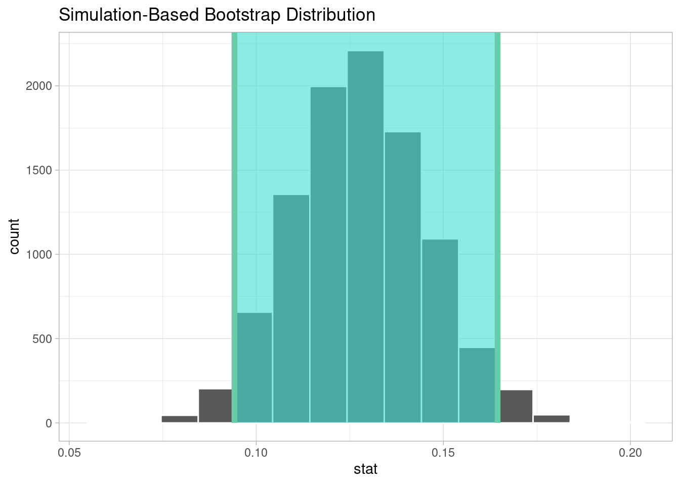
Since the p-value is about 0, we reject the null hypothesis in favor of the alternative hypothesis: the difference between the proportion of popular songs from familiar artists and the proportion of popular songs from unfamiliar artists does not equal zero. The data provides convincing evidence that artists with listeners who are familiar with the artist either have a lower or higher proportion of popular songs than artists that are unfamiliar to listeners.
Analysis 3:
Our third analysis builds off of the second one, except this time we are conducting a one–sided hypothesis test to determine the direction of the difference between song popularity correlated with familiar and unfamiliar artists. Specifically, we conduct a hypothesis test to test if higher artist familiarity is correlated with higher song popularity.
1) Null hypothesis:
\[ p_{familiar} - p_{unfamiliar} = 0 \]
The difference between the proportion of popular songs from familiar artists and the proportion of popular songs from unfamiliar artists equals zero.
2) Alternative hypothesis:
\[ p_{familiar} - p_{unfamiliar} > 0 \]
The difference between the proportion of popular songs from familiar artists and the proportion of popular songs from unfamiliar artists is greater than zero.
Warning in min(diff(unique_loc)): no non-missing arguments to min; returning Inf
Warning: Please be cautious in reporting a p-value of 0. This result is an
approximation based on the number of `reps` chosen in the `generate()` step. See
`?get_p_value()` for more information.
# A tibble: 1 × 1
p_value
<dbl>
1 0# A tibble: 1 × 2
lower_ci upper_ci
<dbl> <dbl>
1 0.0916 0.165
Since the p-value is about 0, we reject the null hypothesis in favor of the alternative hypothesis that the difference between the proportion of popular songs from familiar artists and the proportion of popular songs from unfamiliar artists is greater than zero. The data provides convincing evidence that artists with listeners who are familiar with the artist have a higher proportion of popular songs than artists that are unfamiliar to listeners.
As higher artist familiarity has an association with more song popularity, a factor in growing as in artist is growing in listener retention rate. Listeners who continuously listen to an artist’s songs will be familiar with the artist.
Interpretation and conclusions
Looking at our data analysis, one of our scatter plots explores the relationship between song duration (in seconds) and song hotness. For the most part, song duration, the length of a song does not seem to have an effect on how popular the song is later because most songs are relatively the same length. The hottest songs are usually 240 seconds long. The peak of song hotness occurs at 229.80 seconds. These two variables have a parabolic shape.
Another scatter plot compares song tempo and song hotness. If a song has a tempo of 0 BPM, the hotness is expected to be 0.40, on average. For each increase in song tempo, the song hotness is expected to be higher by 0.00043, on average. There is a extremely slight positive correlation between song tempo and song hotness.
Our interactive model which takes into account song tempo and song duration in relation to song hotness shows us that song tempo and song duration positively affect song hotness to a very slight degree. Through our data analysis we determined that song tempo and duration don’t explain the response variable of song popularity, artist popularity and familiarity do have a relationship with song popularity. From this data we collected we believe that artists and music labels should focus on building their popularity and retention listening rates to increase their song popularity. We even connect this data to Slope Day 2023, where we see that while most people we talked to know at least one of COINS songs people are not familiar with the group themselves.
Limitations
While analyzing our dataset, we encountered a few limitations that we wanted to share:
We noticed a significant number of zero values in our dataset, which we had to remove since it’s impossible for a song to have zero values for variables like song tempo and song duration. Unfortunately, this removal resulted in a reduced number of songs available for analysis and visualization.
Additionally, we found a considerable number of n/a values in the dataset, rendering those songs unusable for our analysis.
The Million Song Data set we used is derived from Echo Nest, the parent company of Spotify, which mainly includes data from Spotify. Therefore, we can assume that the dataset has limited music from other popular streaming platforms like Apple Music, Pandora, or SoundCloud.
Lastly, we observed that the data only goes up to 2011, which makes it less current than desired for some purposes.
Acknowledgments
We are all so grateful to take this class and have the opportunity to learn more about the basics of data science. We send so much love to our TAs and Professor Soltoff. We went to Professor Soltoff’s office hours for advice on our graphs and analyses which was super helpful to gauge our performance on this project. Thank you for providing us with helpful class content to complete this project. Using given resources, we found this data set, allowing us to find useful insights regarding song popularity. All of our information about our data set was from the Million Song Data set and its website.