# load package

library(readr)
library(tidyverse)
library(scales)Marvelous Buneary
Data Collection and Exploratory Data Analysis
Research question(s)
Research question(s). State your research question (s) clearly.
We are planning to research if the referees actually pose impact the result of the game. We plan to categorize the referees by how many yellow/red cards they give during play, preferences for clubs if there are any, and how much extended time they offer and compare these data to the average winning rate of the club to the winning rate of the clubs with the referee
This research will help us understand the impact of subjective views of referees to the game. Potential hypothesis could be “referees have preference for the team and increase the winning rate of such teams.”
Implementation of both categorical and quantitative data will be necessary. We will need to study more about each referee by how strict they are in calling fouls, giving yellow or red cards, and adding extension times. Then, we must compare this to a quantitative variable such as the average winning rate of the club vs that of when a specific referees are in charge.
Data collection and cleaning
Have an initial draft of your data cleaning appendix. Document every step that takes your raw data file(s) and turns it into the analysis-ready data set that you would submit with your final project. Include text narrative describing your data collection (downloading, scraping, surveys, etc) and any additional data curation/cleaning (merging data frames, filtering, transformations of variables, etc). Include code for data curation/cleaning, but not collection.
Load Packages
Downloading all files from reputable source
# load and clean data

epl_record_2000 <- read.csv("data/epl/2000-01.csv") |>
  select(Div, Date, HomeTeam, AwayTeam, FTHG, FTAG, FTR, Referee, HY, AY, HR, AR)
epl_record_2001 <- read.csv("data/epl/2001-02.csv") |>
  select(Div, Date, HomeTeam, AwayTeam, FTHG, FTAG, FTR, Referee, HY, AY, HR, AR)
epl_record_2002 <- read.csv("data/epl/2002-03.csv") |>
  select(Div, Date, HomeTeam, AwayTeam, FTHG, FTAG, FTR, Referee, HY, AY, HR, AR)
epl_record_2003 <- read.csv("data/epl/2003-04.csv") |>
  select(Div, Date, HomeTeam, AwayTeam, FTHG, FTAG, FTR, Referee, HY, AY, HR, AR)
epl_record_2004 <- read.csv("data/epl/2004-05.csv") |>
  select(Div, Date, HomeTeam, AwayTeam, FTHG, FTAG, FTR, Referee, HY, AY, HR, AR)
epl_record_2005 <- read.csv("data/epl/2005-06.csv") |>
  select(Div, Date, HomeTeam, AwayTeam, FTHG, FTAG, FTR, Referee, HY, AY, HR, AR)
epl_record_2006 <- read.csv("data/epl/2006-07.csv") |>
  select(Div, Date, HomeTeam, AwayTeam, FTHG, FTAG, FTR, Referee, HY, AY, HR, AR)
epl_record_2007 <- read.csv("data/epl/2007-08.csv") |>
  select(Div, Date, HomeTeam, AwayTeam, FTHG, FTAG, FTR, Referee, HY, AY, HR, AR)
epl_record_2008 <- read.csv("data/epl/2008-09.csv") |>
  select(Div, Date, HomeTeam, AwayTeam, FTHG, FTAG, FTR, Referee, HY, AY, HR, AR)
epl_record_2009 <- read.csv("data/epl/2009-10.csv") |>
  select(Div, Date, HomeTeam, AwayTeam, FTHG, FTAG, FTR, Referee, HY, AY, HR, AR)
epl_record_2010 <- read.csv("data/epl/2010-11.csv") |>
  select(Div, Date, HomeTeam, AwayTeam, FTHG, FTAG, FTR, Referee, HY, AY, HR, AR)
epl_record_2011 <- read.csv("data/epl/2011-12.csv") |>
  select(Div, Date, HomeTeam, AwayTeam, FTHG, FTAG, FTR, Referee, HY, AY, HR, AR)
epl_record_2012 <- read.csv("data/epl/2012-13.csv") |>
  select(Div, Date, HomeTeam, AwayTeam, FTHG, FTAG, FTR, Referee, HY, AY, HR, AR)
epl_record_2013 <- read.csv("data/epl/2013-14.csv") |>
  select(Div, Date, HomeTeam, AwayTeam, FTHG, FTAG, FTR, Referee, HY, AY, HR, AR)
epl_record_2014 <- read.csv("data/epl/2014-15.csv") |>
  select(Div, Date, HomeTeam, AwayTeam, FTHG, FTAG, FTR, Referee, HY, AY, HR, AR)
epl_record_2015 <- read.csv("data/epl/2015-16.csv") |>
  select(Div, Date, HomeTeam, AwayTeam, FTHG, FTAG, FTR, Referee, HY, AY, HR, AR)
epl_record_2016 <- read.csv("data/epl/2016-17.csv") |>
  select(Div, Date, HomeTeam, AwayTeam, FTHG, FTAG, FTR, Referee, HY, AY, HR, AR)
epl_record_2017 <- read.csv("data/epl/2017-18.csv") |>
  select(Div, Date, HomeTeam, AwayTeam, FTHG, FTAG, FTR, Referee, HY, AY, HR, AR)
epl_record_2018 <- read.csv("data/epl/2018-19.csv") |>
  select(Div, Date, HomeTeam, AwayTeam, FTHG, FTAG, FTR, Referee, HY, AY, HR, AR)
epl_record_2019 <- read.csv("data/epl/2019-20.csv") |>
  select(Div, Date, HomeTeam, AwayTeam, FTHG, FTAG, FTR, Referee, HY, AY, HR, AR)
epl_record_2020 <- read.csv("data/epl/2020-2021.csv") |>
  select(Div, Date, HomeTeam, AwayTeam, FTHG, FTAG, FTR, Referee, HY, AY, HR, AR)
epl_record_2021 <- read.csv("data/epl/2021-2022.csv") |>
  select(Div, Date, HomeTeam, AwayTeam, FTHG, FTAG, FTR, Referee, HY, AY, HR, AR)
# merge data
epl <- rbind(epl_record_2000, epl_record_2001, epl_record_2002,
epl_record_2003, epl_record_2004, epl_record_2005,
epl_record_2006, epl_record_2007, epl_record_2008,
epl_record_2009, epl_record_2010, epl_record_2011,
epl_record_2012, epl_record_2013, epl_record_2014,
epl_record_2015, epl_record_2016, epl_record_2017,
epl_record_2018, epl_record_2019, epl_record_2020,
epl_record_2021)# glimpse data
glimpse(epl)Rows: 8,020
Columns: 12
$ Div <chr> "E0", "E0", "E0", "E0", "E0", "E0", "E0", "E0", "E0", "E0", "…
$ Date <chr> "19/08/00", "19/08/00", "19/08/00", "19/08/00", "19/08/00", "…
$ HomeTeam <chr> "Charlton", "Chelsea", "Coventry", "Derby", "Leeds", "Leicest…
$ AwayTeam <chr> "Man City", "West Ham", "Middlesbrough", "Southampton", "Ever…
$ FTHG <int> 4, 4, 1, 2, 2, 0, 1, 1, 3, 2, 2, 2, 1, 1, 3, 4, 3, 1, 0, 5, 0…
$ FTAG <int> 0, 2, 3, 2, 0, 0, 0, 0, 1, 0, 0, 0, 1, 1, 0, 2, 2, 2, 1, 3, 0…
$ FTR <chr> "H", "H", "A", "D", "H", "D", "H", "H", "H", "H", "H", "H", "…
$ Referee <chr> "Rob Harris", "Graham Barber", "Barry Knight", "Andy D'Urso",…
$ HY <int> 1, 1, 5, 1, 1, 2, 1, 3, 0, 0, 2, 0, 1, 2, 2, 3, 0, 5, 3, 0, 1…
$ AY <int> 2, 2, 3, 1, 3, 3, 1, 1, 0, 1, 4, 1, 4, 1, 1, 3, 3, 3, 3, 1, 2…
$ HR <int> 0, 0, 1, 0, 0, 0, 0, 0, 0, 0, 1, 0, 0, 0, 0, 0, 1, 0, 1, 0, 0…
$ AR <int> 0, 0, 0, 0, 0, 0, 0, 1, 0, 0, 2, 0, 0, 0, 1, 0, 0, 0, 0, 0, 0…Data description
Have an initial draft of your data description section. Your data description should be about your analysis-ready data.
QUESTIONS TO ANSWER:
What are the observations (rows) and the attributes (columns)?
- There are 8020 observations (rows) and 12 attributes (columns) in this data set.
Why was this data set created?
- Football (Soccer) is played and watched by millions all over the world, and as a result, sports betting has become an incredibly profitable market. The English Premier League, in particular, is the world’s most popular domestic team. As a result, this data set curated the Premier League’s matches from the past 20 years in order to make predictive analysis towards future games, and aid in sports betting.
Who funded the creation of the data set?
- While there is no information provided as to who funded the creation of the data set, it was collected and curated by Saif Uddin.
What processes might have influenced what data was observed and recorded and what was not?
- Significant factors that influenced what data was recorded were the statistics available. The present data set only comprises of match statistics that were made available to the curator.
What pre-processing was done, and how did the data come to be in the form that you are using?
The original data was collected from “http://football-data.co.uk”, after which it was cleaned by the curator. To make this data set usable, the curator filtered through instances of old book markers/ abbreviations no longer presently relevant and appended a current list of book markers for the data set. Also, in the event of missing instances of specific Fouls data (France 2nd, Belgium 1st, and Greece 1st divisions), the original curator processed them as ‘Free Kicks Conceded’ as this connotation includes references to fouls not stated.
To make the data set useful for our analysis, the data was narrowed down and filtered to include only informational match and referee data, including:
Div = League Division
Date = Match Date (dd/mm/yy)
HomeTeam = Home Team
AwayTeam = Away Team
FTHG = Full Time Home Team Goals
FTAG = Full Time Away Team Goals
FTR = Full-Time Result (H=Home Win, D=Draw, A=Away Win)
Referee = Match Referee
HY = Home Team Yellow Cards
AY = Away Team Yellow Cards
HR = Home Team Red Cards
AR = Away Team Red Cards
If people are involved, were they aware of the data collection and if so, what purpose did they expect the data to be used for?
- No, people aren’t involved as the data was (and is) curated from “http://football-data.co.uk”.
Data limitations
Identify any potential problems with your data set.
- There are no significant problems except for the fact that the data set may not be representative of more recent matches past 2022.
Exploratory data analysis
Perform an (initial) exploratory data analysis.
# (1) Who are the more experienced referees with over 100 matches?
epl_exp_ref <- epl |>
  group_by(Referee) |>
  count() |>
  ungroup() |>
  filter(n > 100) |>
  arrange(desc(n))
epl_exp_ref
# A tibble: 25 × 2
Referee n
<chr> <int>
1 M Dean 505
2 M Atkinson 433
3 A Marriner 356
4 P Dowd 301
5 H Webb 296
6 M Clattenburg 293
7 M Oliver 291
8 A Taylor 286
9 L Mason 274
10 C Foy 256
# ℹ 15 more rows# (2) How do referees tend to impact the result of a match?
## filter for only experienced referees with over 100 matches
## wrangle data to have an idea of the general distribution
epl |>
filter(Referee %in% epl_exp_ref$Referee) |>
group_by(Referee, FTR) |>
summarize(count = n()) |>
ungroup() |>
pivot_wider(
names_from = "FTR",
values_from = "count") |>
arrange(desc(H)) |>
mutate(Total = A + D + H) |>
mutate(pctH = H / Total,
pctD = D / Total,
pctA = A / Total) |>
relocate(Referee, Total, H, D, A) # A tibble: 25 × 8
Referee Total H D A pctH pctD pctA
<chr> <int> <int> <int> <int> <dbl> <dbl> <dbl>
1 M Dean 505 216 146 143 0.428 0.289 0.283
2 M Atkinson 433 198 100 135 0.457 0.231 0.312
3 A Marriner 356 154 88 114 0.433 0.247 0.320
4 P Dowd 301 145 75 81 0.482 0.249 0.269
5 L Mason 274 138 62 74 0.504 0.226 0.270
6 M Clattenburg 293 138 76 79 0.471 0.259 0.270
7 H Webb 296 133 83 80 0.449 0.280 0.270
8 C Foy 256 128 57 71 0.5 0.223 0.277
9 M Oliver 291 128 78 85 0.440 0.268 0.292
10 A Taylor 286 124 67 95 0.434 0.234 0.332
# ℹ 15 more rows## visualization of how referees tend to impact the result of a match
epl |>
filter(Referee %in% epl_exp_ref$Referee) |>
group_by(Referee, FTR) |>
summarize(count = n()) |>
ungroup() |>
ggplot(mapping = aes(y = Referee, x = count, fill = FTR)) +
geom_col(position = "fill") +
guides(fill = guide_legend(reverse = TRUE)) +
labs(
title = "How EPL referees tend to impact the result of a match",
subtitle = "(sampled only experienced referees with over 100 matches)",
x = "Number of Matches",
y = "Referee Name",
fill = "Full-Time Result",
caption = "Data Source: http://football-data.co.uk"
) +
scale_x_continuous(labels = label_percent()) +
scale_fill_viridis_d(option = "D", begin = 0.1,
labels = c("Away Win", "Draw", "Home Win")) +
theme_minimal() +
theme(plot.title = element_text(size = 12, face = "bold", hjust = 0),
plot.title.position = "plot",
legend.position = "bottom")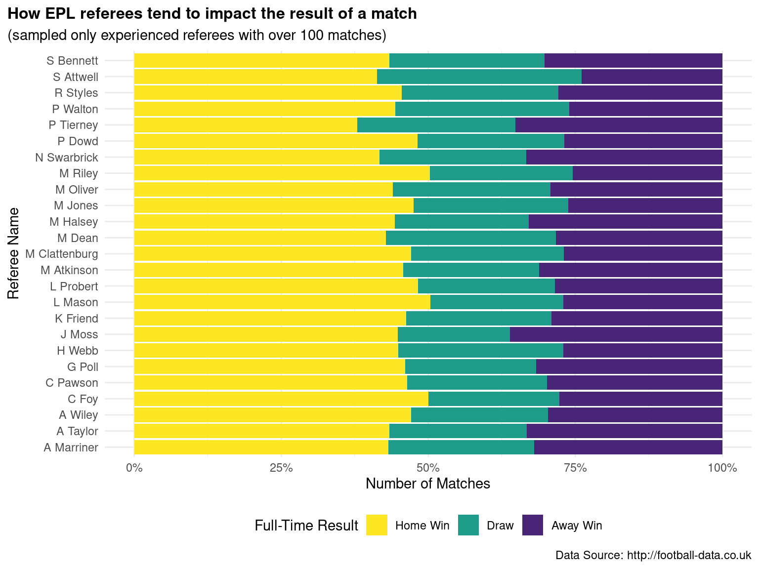
# (3) Which experienced referees gave the most red cards during a play, on average, for both the Home Team and Away Team?
epl |>
  group_by(Referee) |>
  summarise(count = n(),
            mean_HR = mean(HR),
            mean_AR = mean(AR)) |>
  mutate(mean_Red = mean_HR + mean_AR) |>
  ungroup() |>
  filter(count >= 100) |>
  relocate(Referee, mean_Red, mean_HR, mean_AR, count) |>
  arrange(desc(mean_Red))
# A tibble: 25 × 5
Referee mean_Red mean_HR mean_AR count
<chr> <dbl> <dbl> <dbl> <int>
1 R Styles 0.284 0.114 0.170 176
2 P Dowd 0.216 0.0764 0.140 301
3 M Riley 0.213 0.112 0.101 169
4 M Dean 0.204 0.0733 0.131 505
5 S Bennett 0.2 0.0537 0.146 205
6 L Probert 0.174 0.0698 0.105 172
7 A Marriner 0.163 0.0618 0.101 356
8 M Clattenburg 0.160 0.102 0.0580 293
9 M Atkinson 0.150 0.0647 0.0855 433
10 C Pawson 0.149 0.0663 0.0829 181
# ℹ 15 more rows# (4) Which experienced referees gave the most yellow cards during a play, on average, for both the Home Team and Away Team?
epl |>
group_by(Referee) |>
summarise(count = n(),
mean_HY = mean(HY),
mean_AY = mean(AY)) |>
mutate(mean_Yellow = mean_HY + mean_AY) |>
ungroup() |>
filter(count >= 100) |>
relocate(Referee, mean_Yellow, mean_HY, mean_AY, count) |>
arrange(desc(mean_Yellow))# A tibble: 25 × 5
Referee mean_Yellow mean_HY mean_AY count
<chr> <dbl> <dbl> <dbl> <int>
1 M Dean 3.65 1.78 1.88 505
2 M Riley 3.60 1.56 2.04 169
3 C Pawson 3.58 1.71 1.87 181
4 S Attwell 3.56 1.73 1.83 138
5 P Dowd 3.54 1.45 2.09 301
6 S Bennett 3.51 1.46 2.04 205
7 K Friend 3.44 1.65 1.80 251
8 A Taylor 3.42 1.66 1.76 286
9 P Tierney 3.39 1.62 1.77 108
10 N Swarbrick 3.33 1.67 1.67 132
# ℹ 15 more rowsQuestions for reviewers
List specific questions for your peer reviewers and project mentor to answer in giving you feedback on this phase.
What degree of certainty do we need to claim referee bias or support?
Are there any factors seen in our data set that would be helpful to include?