Accident Severity in New York State

Report based on recorded vehicle accidents (2016-2021)

Introduction

Severe vehicular accidents are a leading cause of non-natural injuries and death in the United States. As such, our team sought to look more deeply into this issue affecting our society. We were motivated in our data exploration to identify the conditions linked to more severe accidents in hopes of using this information to help emergency responders and other related services better anticipate future accidents and be able to prepare their resources accordingly. We chose to explore data regarding some of these traffic accidents in hopes of answering the following question: is there a relationship between driving conditions and the severity of traffic accidents, and if so, what are the driving conditions that correlate to more severe accidents? Through our analysis, we discovered that wind speed and precipitation significantly impact accident severity, whereas time of accident (day/night) had no significant effect on accident severity. While a majority of this report focuses on the general predictors of accident severity, we also included an additional analysis on accident severity in Tompkins County as it relates to Cornell University students.

Data description

Our data comes from a large traffic accident dataset containing over 2.8 million observations from 49 U.S. states, where each observation (row) is a traffic accident. Each accident has recorded details (columns) such as the date/time, location, severity, weather conditions, cause of incident, and other information.

This dataset was collected in real time between February 2016 and December 2021 using multiple APIs that provide streaming traffic incident (or event) data. The traffic data comes from a variety of sources, such as the U.S. and state departments of transportation, law enforcement agencies, traffic cameras, and traffic sensors within the road-networks.

The data set collection was supported by a grant from the Ohio Supercomputer Center (PAS0536), and this dataset was assembled by Lyft data scientists Sobhan Moosavi, Mohammad Hossein Samavatian, Srinivasan Parthasarathy, and Rajiv Ramnath. Their goal is to help solve the public safety challenge of reducing traffic accidents by providing a public, up-to-date, and large-scale dataset that can be used to perform studies on traffic accident analysis and prediction.

To narrow down the scope of the data and to be able to perform faster processing, we chose to only include observations from New York for this project. We also chose to only look at the four most common types of “Accident Infrastructure” variables as many indicators were only present in <1% of observations.

We also excluded additional extraneous accident details, such as variables surrounding the exact accident location and weather variables irrelevant to our primary analysis as part of our data cleaning. Full data cleaning scripts and further justification for the exclusion of certain variables are included in the data cleaning appendix.

Data analysis

In the data analysis section we have two main goals. The first is to develop multiple logistic regression models that show the relationship between an accident being considered severe and corresponding explanatory variables. We choose to focus on this to seek answers to the global question of what is behind severe car accidents. The second is to determine whether or not there is a statistically significant difference between severe accidents in Tompkins county at day and at night. We choose to focus on this because it pertains to our every day lives.

Sampling Severity

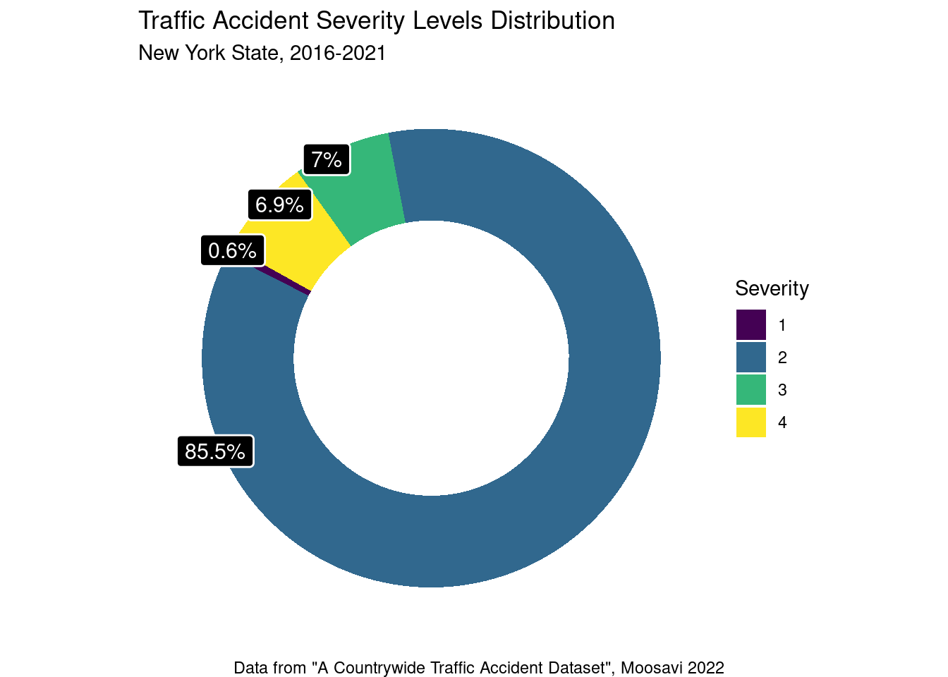
Given that severity will be the outcome variable in our logistic regression models, it is important to first understand the distribution of accidents into the severity categories. When looking at the data, we initially observed a problem with the New York data where the vast majority (85.5%) of accidents were rated with a severity of 2.

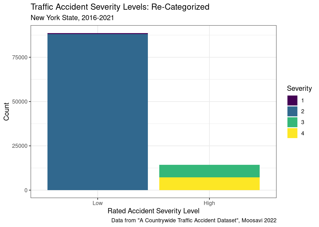
Having the vast majority of data in one severity level is problematic for models that predict severity as they would be biased and better at identifying accidents in severity level 2. To combat this issue, the data was first re-categorized into two severity levels. Accidents falling into the severity levels 1 and 2 were combined, representing accidents that have a low severity. Accidents falling into the severity levels 3 and 4 were combined, representing accidents that have a high severity.

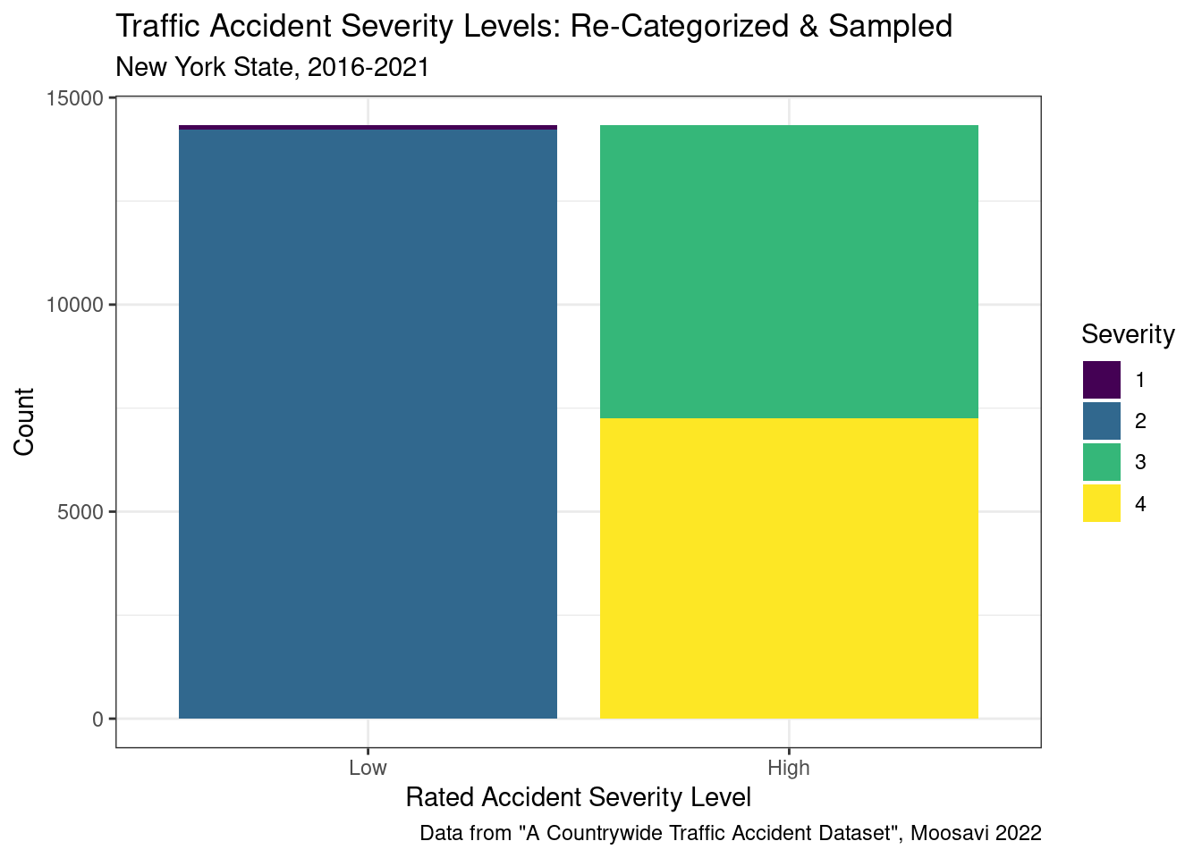
Then, to further balance the data, random sampling was used, where a random sample was taken from the Low severity category to equal the number of observations in the High category (14,334). In sum, the sampled dataset contains 28,668 observations, half of which are of high severity and half of which are of low severity. While the majority of accidents are still from severity category 2, the equality between low and high should provide a better balance for the logistic regression models at predicting severity given certain conditions.

Time of Day Analysis in Tompkins County, NY

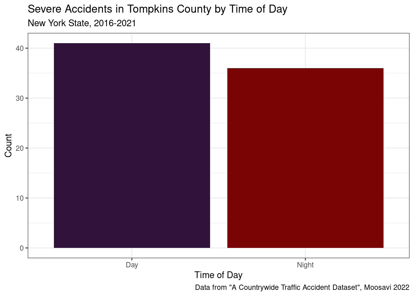
In an application to Cornell students, we will also conduct inference via a hypothesis test to see if the proportion of severe accidents in Tompkins County is statistically significantly different at the 95% level between day time and night time. The data was prepped for Tompkins County by factoring, filtering, and again re-categorizing the severity level to conduct such inference and allows us to visualize the apparent difference in severe accidents at day and at night:

Modeling

Now to do our logistic regression, there is one last modification that needs to be made to our data. Our outcome variable currently has two levels (high and low) that are characters. We will thus create a new variable with a 0 representing a “low” accident and a 1 representing a “high” accident. This will allow the computer to run the logistic regression. Furthermore, we will convert this variable to a factor so that we can utilize it as the outcome variable in our logit models.

[1] "numeric"

[1] "factor"

Note: In each model p represents the probability of accident being considered severe

# A tibble: 4 × 5
  term              estimate std.error statistic   p.value
  <chr>                <dbl>     <dbl>     <dbl>     <dbl>
1 (Intercept)       -0.404     0.0471      -8.58 9.42e- 18
2 Precipitation.in.  0.421     0.0149      28.3  2.27e-176
3 Visibility.mi.    -0.00604   0.00448     -1.35 1.78e-  1
4 Wind_Speed.mph.    0.0360    0.00218     16.5  1.82e- 61

\[ \begin{equation*} \begin{aligned} \ln[p\ /\ (1-p)] = -0.404 + 0.42 \times \text{Precipitation.in} \ - \\ 0.006 \times \text{Visibility.mi} + 0.036 \times \text{WindSpeed.mph} \end{aligned} \end{equation*} \]

# A tibble: 8 × 5
  term                           estimate std.error statistic   p.value
  <chr>                             <dbl>     <dbl>     <dbl>     <dbl>
1 (Intercept)                    -0.416     0.0509     -8.18  2.84e- 16
2 Precipitation.in.               0.464     0.0174     26.7   1.51e-157
3 JunctionTRUE                    0.102     0.134       0.758 4.49e-  1
4 Visibility.mi.                 -0.00474   0.00484    -0.978 3.28e-  1
5 Wind_Speed.mph.                 0.0374    0.00237    15.8   6.83e- 56
6 Precipitation.in.:JunctionTRUE -0.190     0.0343     -5.54  2.94e-  8
7 JunctionTRUE:Visibility.mi.    -0.0114    0.0129     -0.888 3.75e-  1
8 JunctionTRUE:Wind_Speed.mph.   -0.00860   0.00600    -1.43  1.52e-  1

\[ \begin{split} \\ln[p\ /\ (1-p)] = -0.416 + 0.464 \times Precipitation.in \ + \\0.102 \times Junction - 0.005 \times Visibility.mi \ + \\ 0.037 \times WindSpeed.mph \ - \\0.190 \times Junction \times Precipitation.in \ - \\0.011 \times Junction \times Visibility.mi \ - \\ 0.009 \times Junction \times WindSpeed.mph \end{split} \]

Evaluation of significance

Logistic Regression Models

While the tidy function used above extracts p-values and test statistics for each model, we wanted to take a more robust approach to verify the statistical significance of our coefficient values. The code chunks below generate a null distribution and calculate p-values based on the observed model’s coefficients in comparison to the null distribution. This approach might be better than just pulling values from the above tables as it provides a non-parametric approach to calculate p-values and does not rely on specific assumptions about the distribution of the data. Furthermore, the code chunks below calculate confidence intervals for coefficient and intercept values. Nevertheless, both methods yield similar results in terms of p-values and identical results in terms of which coefficients are statistically significant and which are not.

Additive Logit Model:

# A tibble: 4 × 3
  term              lower_ci upper_ci
  <chr>                <dbl>    <dbl>
1 Precipitation.in. -0.0243   0.0203 
2 Visibility.mi.    -0.00840  0.00864
3 Wind_Speed.mph.   -0.00400  0.00436
4 intercept         -0.0885   0.0827

# A tibble: 4 × 2
  term              p_value
  <chr>               <dbl>
1 Precipitation.in.   0    
2 Visibility.mi.      0.172
3 Wind_Speed.mph.     0    
4 intercept           0

Interactive Logit Model:

# A tibble: 8 × 3
  term                            lower_ci upper_ci
  <chr>                              <dbl>    <dbl>
1 JunctionFALSE                    -0.244    0.242 
2 JunctionFALSE:Visibility.mi.     -0.0232   0.0232
3 JunctionFALSE:Wind_Speed.mph.    -0.0118   0.0124
4 Precipitation.in.                -0.0523   0.0501
5 Precipitation.in.:JunctionFALSE  -0.0578   0.0546
6 Visibility.mi.                   -0.0215   0.0223
7 Wind_Speed.mph.                  -0.0111   0.0105
8 intercept                        -0.230    0.225

# A tibble: 8 × 2
  term                            p_value
  <chr>                             <dbl>
1 JunctionFALSE                     0.39 
2 JunctionFALSE:Visibility.mi.      0.328
3 JunctionFALSE:Wind_Speed.mph.     0.142
4 Precipitation.in.                 0    
5 Precipitation.in.:JunctionFALSE   0    
6 Visibility.mi.                    0.162
7 Wind_Speed.mph.                   0    
8 intercept                         0.012

Tompkins County Severity of Accident Hypothesis Test:

For the second part of our analysis we performed a hypothesis test to assess whether there is a significant difference in the proportion of high severity accidents between day and night.

# A tibble: 1 × 1
  p_value
    <dbl>
1   0.078

Interpretation and conclusions

Model 1 Interpretations:

When all predictors in the model are equal to zero, we expect the odds of an accident being considered severe to be 0.668 times higher.

For every one inch increase in precipitation, we expect the odds of an accident being considered severe to be 1.524 times higher, holding all other variables constant.

For every one mile increase in visibility, we expect the odds of an accident being considered severe to be 0.994 times higher, holding all other variables constant.

For every one mile per hour increase in wind speed, we expect the odds of an accident being considered severe to be 1.036 times higher, holding all other variables constant.

Model 2 Interpretations:

When all predictors in the model are equal to zero, we expect the odds of an accident being considered severe to be 0.659 times higher.

For every one inch increase in precipitation given that we are at a junction, we expect the odds of an accident being considered severe to be 1.31 times higher, holding all other variables constant.

For every one inch increase in precipitation given that we are not at a junction, we expect the odds of an accident being considered severe to be 1.59 times higher, holding all other variables constant.

For every one mile increase in visibility given that we are at a junction, we expect the odds of an accident being considered severe to be 0.983 times higher, holding all other variables constant.

For every one mile increase in visibility given that we are not at a junction, we expect the odds of an accident being considered severe to be 0.995 times higher, holding all other variables constant.

For every one mile per hour increase in wind speed given that we are at a junction, we expect the odds of an accident being considered severe to be 1.03 times higher, holding all other variables constant.

For every one mile per hour increase in wind speed given that we are not at a junction, we expect the odds of an accident being considered severe to be 1.04 times higher, holding all other variables constant.

Conclusion from additive model:

\[ \begin{split} H_o: \beta_1 = \beta_2 = \beta_3 = 0 \\ H_a: \beta_1 \neq 0 \ or \beta_2 \neq 0 \ or \beta_3 \neq 0 \end{split} \]

Here we have three separate hypothesis tests. Upon running the regression and then confirming our results with re-sampling, we find that the coefficients on precipitation and wind speed have p-values than 0.05, while visibility does not. Therefore, there is sufficient evidence to reject two of the the null hypotheses at the 95% confidence level and conclude that there is a meaningful relationship between accident severity and precipitation and accident severity and wind speed.

Conclusion from interactive model:

\[ \begin{split} H_o: \beta_1 = \beta_2 = \beta_3 = \beta_4 = \beta_5 = \beta_6 = \beta_7 = 0 \\ H_a: \beta_1 \neq 0 \ or \beta_2 \neq 0 \ or \beta_3 \neq 0 \ or \beta_4 \neq0 \ or \beta_5 \neq 0 \ or \beta_6 \neq 0 \ or \beta_7 \neq 0 \end{split} \]

Here we have seven separate hypothesis tests. Upon running the regression and then confirming our results with re-sampling, we find that the coefficients on precipitation, wind speed, and the interaction between precipitation and junction have p-values than 0.05, while all other variables do not. Therefore, there is sufficient evidence to reject three of the null hypotheses at the 95% confidence level and conclude that there is a meaningful relationship between accident severity and precipitation, accident severity and wind speed, as well as a significant interaction between precipitation and junction.

Conclusion from Tompkins County Hypothesis Test:

\[ \begin{split} H_0: P_{Day} - P_{Night} = 0 \\ H_a: P_{Day} - P_{Night} \neq 0 \end{split} \]Is the true proportion of high severity accidents in Tompkins county different during the day and the night? Given the p-value of .078 is greater than .05, we fail to reject the null hypothesis at the 95% significance level. Therefore, we can conclude that there is not a statistically significant difference in the proportion of severe accidents during the day vs the night in Tompkins county.

Limitations

We have identified two main limitations with our data:

Outcome variable of severity: There are several issues with our outcome variables regarding severity. Firstly, severity is currently measured on a scale of 1 to 4. However, in order to use it in our model, we will have to classify accidents as more or less severe by grouping 1 and 2 as 0, and 3 and 4 as 1 to perform logistic regression. This has the potential to impact the precision of our model. Furthermore, severity is measured in terms of its impact on traffic, specifically the time it takes for the accident to be cleared. While this measure is often significantly correlated with actual severity, it may not capture more important outcomes such as injuries, loss of life, or monetary damage to vehicles.
Use of NY State: When using data from NY state alone to determine the factors that influence accident severity, several potential issues may arise. Firstly, the results obtained may not be generalizable to other regions or countries, as the factors that affect accident severity may differ. Secondly, the sample size may be small for an experiment like this, resulting in low statistical power and difficulties in drawing accurate conclusions. Thirdly, there may be bias in the analysis if the data collected in the dataset is not representative of all accidents in NY state. For instance, we can expect the clean up time for motor vehicle accidents in New York City (and thus the severity variable) to be different from motor vehicle accidents in rural upstate New York as a result of differences in emergency services infrastructure and resources.

The limitations surrounding the way this dataset’s severity outcome variable was measured impacted our ability to draw more specific conclusions regarding the true impact of contributing variables on motor vehicle accidents, and the limitations caused by our use of data collected in New York State exclusively was a potential source of bias when drawing conclusions on New York State accidents.

However, some potential remedies for future iterations of this analysis may include: performing analyses by different New York State zip codes and comparing those results for discrepancies, using data from multiple states and aggregating the conclusions on those analyses, or even finding a different measure of accident severity from another data set (that measures accident severity by a more meaningful measure than clean up time) to be able to make more specific conclusions.

Acknowledgments

We thank the data set author Sobhan Moosavi for allowing the use of this well maintained and high quality data set for our academic and research use. We thank our discussion section TAs and peers for their valuable and constructive feedback in our project journey.