An Exploration of Arabica Coffee and its Attributes
Exploratory data analysis
Research question(s)
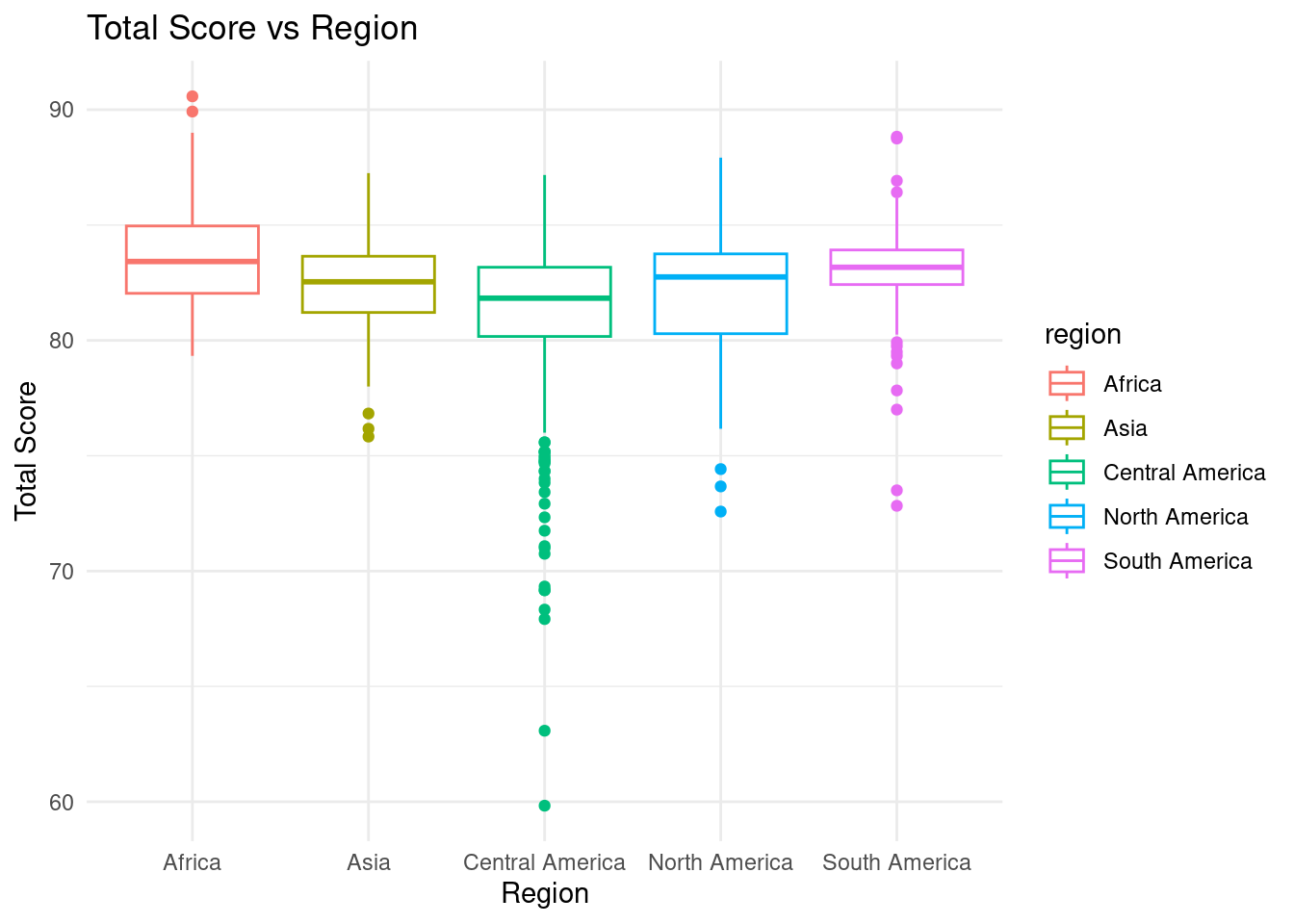
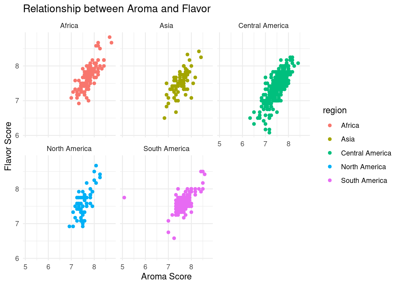
How do Arabica beans from different regions differ in their scores of aroma, flavor, etc? Does region impact the relationship between different scores?
Regions including North America (United States), Central America (Costa Rica, El Salvador, Guatemala, Honduras, Mexico, Nicaragua, Panama, Haiti), South America (dBrazil, Colombia, Ecuador, Peru), Africa (Burundi, Ethiopia, Kenya, Malawi, Rwanda, Tanzania, United Republic Of Uganda, Zambia, Cote d?Ivoire), and Asia (Taiwan, China, India, Thailand, Vietnam, Myanmar, Indonesia, Laos, Philippines, Papau New Guinea)
Data collection and cleaning
Have an initial draft of your data cleaning appendix. Document every step that takes your raw data file(s) and turns it into the analysis-ready data set that you would submit with your final project. Include text narrative describing your data collection (downloading, scraping, surveys, etc) and any additional data curation/cleaning (merging data frames, filtering, transformations of variables, etc). Include code for data curation/cleaning, but not collection.
Attaching package: 'janitor'

The following objects are masked from 'package:stats':

    chisq.test, fisher.test
library(scales)
Attaching package: 'scales'

The following object is masked from 'package:purrr':

    discard

The following object is masked from 'package:readr':

    col_factor
#import data, remove columns not using, change double to numericcoffee <-read_csv("data/coffee.csv", col_types =cols(Location.Region =col_skip(), Location.Altitude.Min =col_skip(), Location.Altitude.Max =col_skip(), Location.Altitude.Average =col_integer(), Year =col_skip(), Data.Owner =col_skip(), `Data.Production.Number of bags`=col_skip(), `Data.Production.Bag weight`=col_skip(), Data.Scores.Aroma =col_number(), Data.Scores.Flavor =col_number(), Data.Scores.Aftertaste =col_number(), Data.Scores.Acidity =col_number(), Data.Scores.Body =col_number(), Data.Scores.Balance =col_number(), Data.Scores.Uniformity =col_number(), Data.Scores.Sweetness =col_number(), Data.Scores.Moisture =col_number(), Data.Color =col_skip()), na ="NA")#clean variable namescoffee <- coffee |>clean_names()#count number of each countrycoffee2 <- coffee |>filter(data_type_species =="Arabica") |>group_by(location_country) |>summarize("country types"=n())#create vectors for each regionnorth_america <-c("United States")central_america <-c("Costa Rica", "El Salvador", "Guatemala", "Honduras", "Mexico", "Nicaragua", "Panama", "Haiti")south_america <-c("Brazil", "Colombia", "Ecuador", "Peru")africa <-c("Burundi", "Ethiopia", "Kenya", "Malawi", "Rwanda", "Tanzania, United Republic Of", "Uganda", "Zambia", "Cote d?Ivoire")asia <-c("Taiwan", "China", "India", "Thailand", "Vietnam", "Myanmar", "Indonesia", "Laos", "Philippines", "Papua New Guinea")#create regions columncoffee_regions <- coffee |>mutate (region =case_when( location_country %in% north_america ~"North America", location_country %in% central_america ~"Central America", location_country %in% south_america ~"South America", location_country %in% africa ~"Africa", location_country %in% asia ~"Asia",TRUE~NA_character_ )) |>relocate(region, .after = location_country) |>filter(data_type_species =="Arabica") |>filter (data_scores_total !=0)#count number of observations for each regioncoffee_reg <- coffee_regions |>filter(data_type_species =="Arabica") |>group_by(region) |>summarize("region amt"=n())
Data description
This data set consists of Arabica coffee beans sorted into five different geographic regions dependent on the country the beans were from. Each observation of coffee beans was given a score from 0-10 regarding flavor, aroma, etc. There are also variables representing the average altitude of the location and the processing method of the beans. The original data set was published by @jthomasmock in his contribution to the TidyTuesday project on Github and is from the CORGIS Dataset Project by Sam Donald, created on July 6, 2020. The dataset is called coffee_regions.
Data limitations
One potential problem with our data set is that each region does not contain the same number of observations. For example, the North America region contains 63 observations while Central America contains 494 observations. However, this can be remedied by finding models that fit each region and thus do not rely on the number of observations. Also another potential problem is having NA values in our data and scores of 0. Thus, to fix this we can filter and drop the na’s.
Exploratory data analysis
Perform an (initial) exploratory data analysis.
#regions-score plot; all have similar median around 82ggplot(data = coffee_regions, mapping =aes(x = region, y = data_scores_total, color = region)) +geom_boxplot() +labs(x ="Region",y ="Total Score",title ="Total Score vs Region") +theme_minimal()
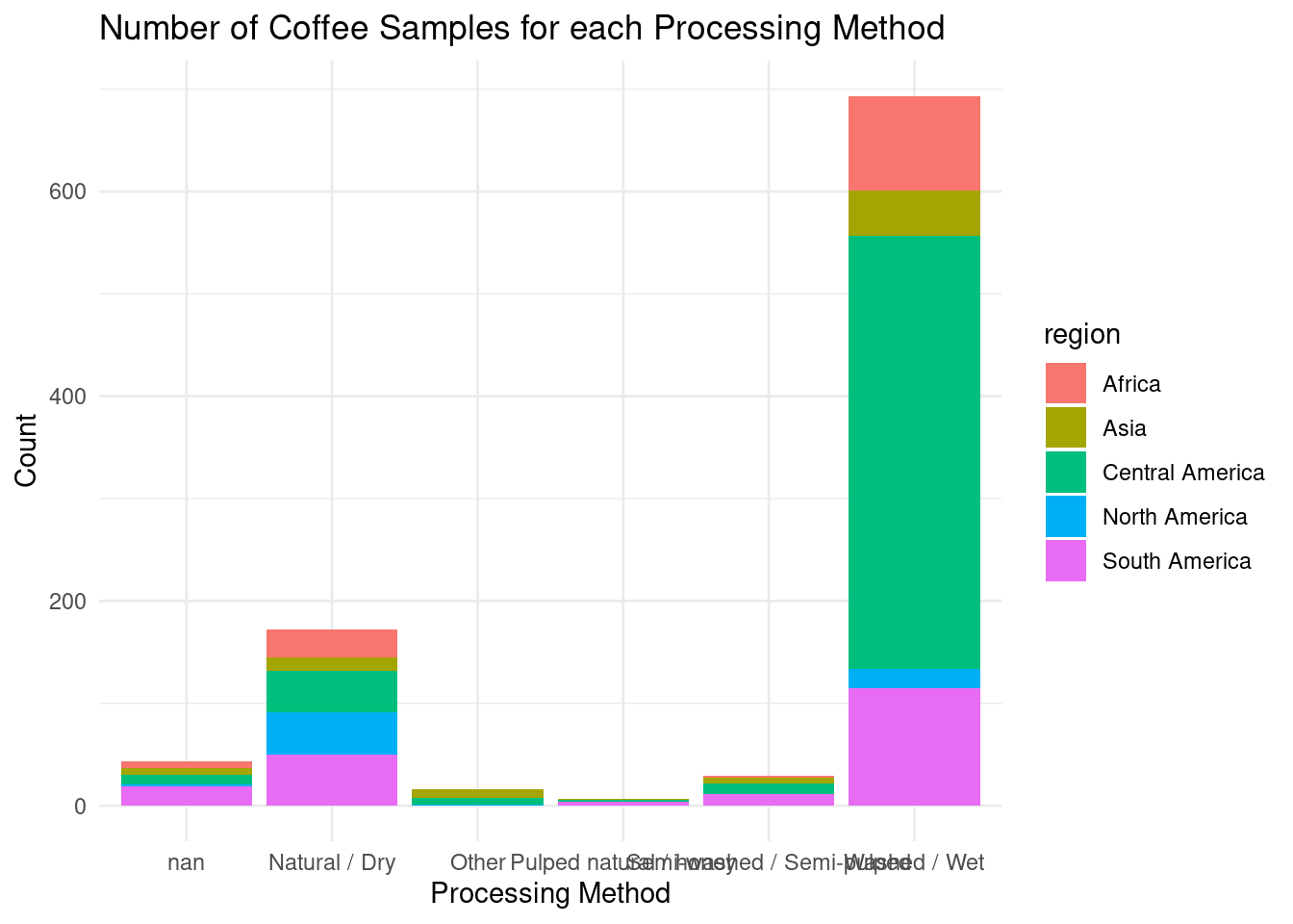
#histogram of processing methodsggplot(data = coffee_regions, aes(x = data_type_processing_method, fill = region)) +geom_bar() +labs(title ="Number of Coffee Samples for each Processing Method",x ="Processing Method",y ="Count" ) +theme_minimal()
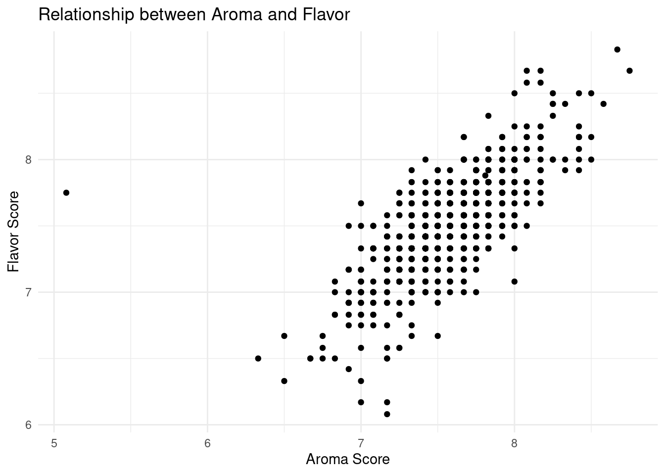
#aroma-flavor scatterplot, positive linear relationshipggplot(data = coffee_regions, mapping =aes(x = data_scores_aroma, y = data_scores_flavor)) +geom_point() +labs(x ="Aroma Score",y ="Flavor Score",title ="Relationship between Aroma and Flavor") +theme_minimal()
#aroma-flavor scatterplot, faceted by regionggplot(data = coffee_regions, mapping =aes(x = data_scores_aroma, y = data_scores_flavor, color = region)) +geom_point() +labs(x ="Aroma Score",y ="Flavor Score",title ="Relationship between Aroma and Flavor") +theme_minimal() +facet_wrap(vars(region))
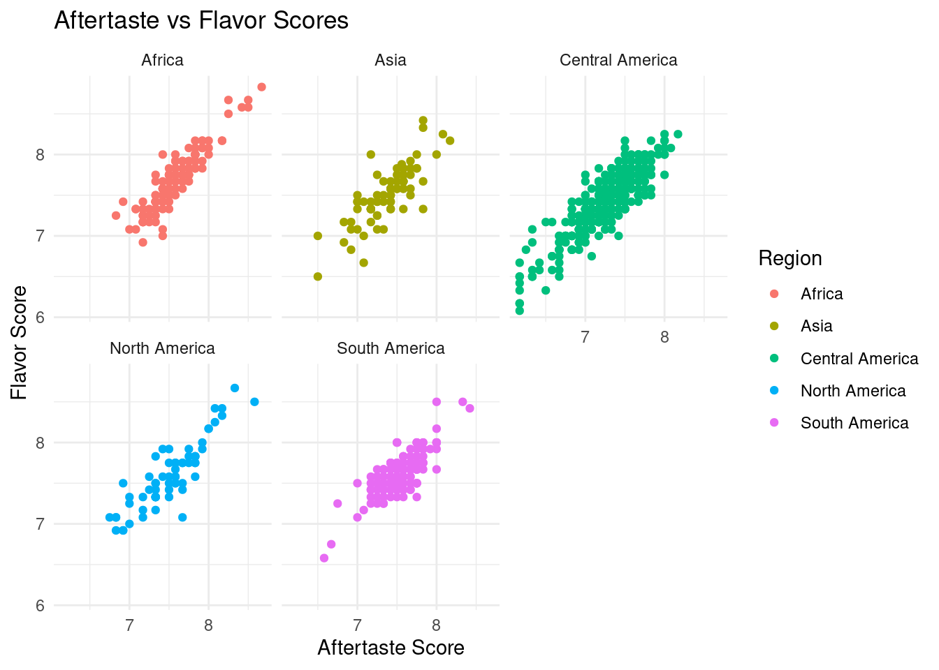
# scatterplot aftertaste-flavor coffee_regions |>ggplot(aes(x = data_scores_aftertaste, y = data_scores_flavor, color = region)) +geom_point() +labs(title ="Aftertaste vs Flavor Scores",x ="Aftertaste Score",y ="Flavor Score",color ="Region") +theme(legend.position ="bottom") +facet_wrap(vars(region)) +theme_minimal()
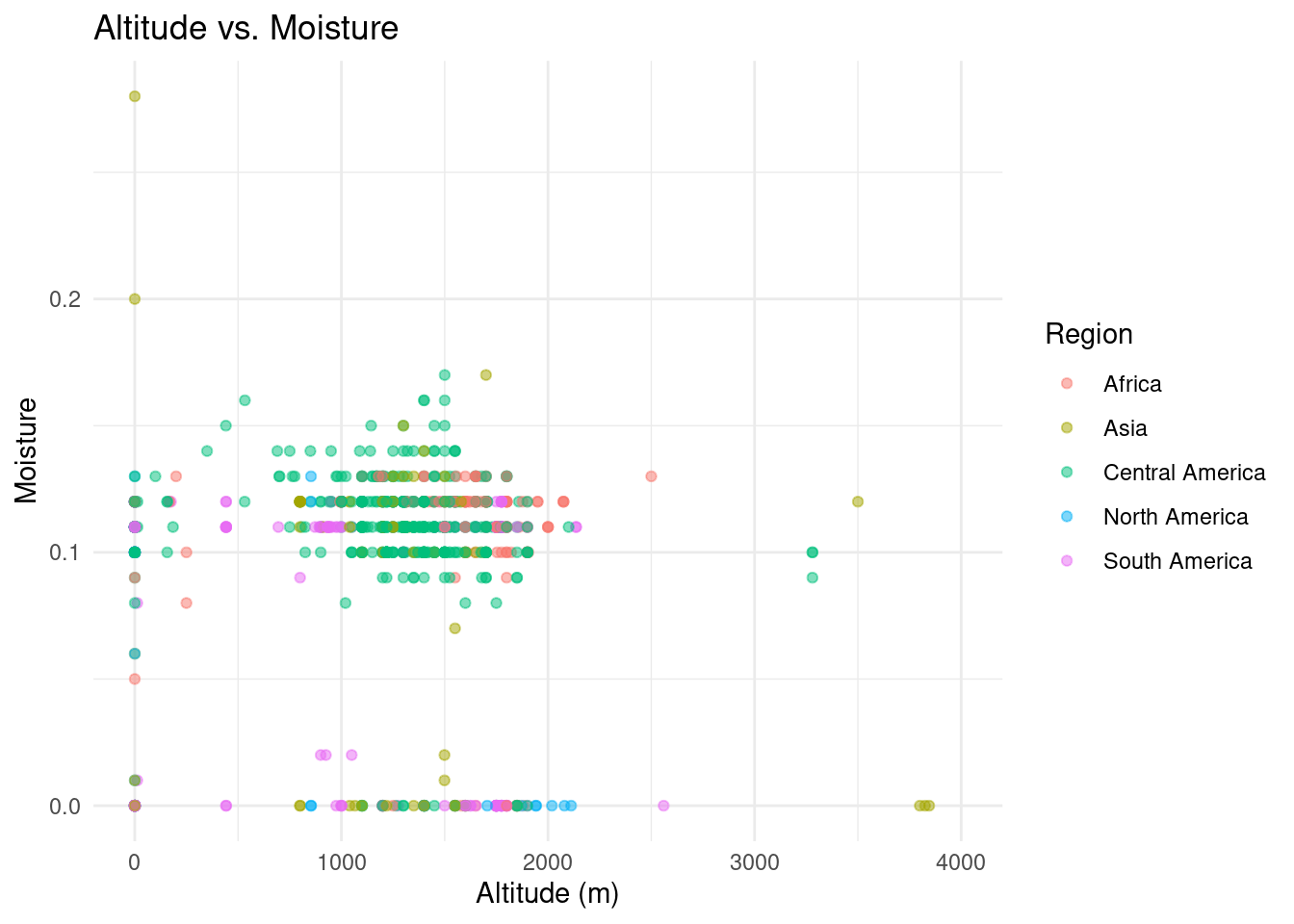
#scatter plot of altitude vs moisture score; no obvious correlationggplot(data = coffee_regions, mapping =aes(x = location_altitude_average, y = data_scores_moisture, color = region)) +geom_point(alpha =0.5) +labs(title ="Altitude vs. Moisture", x ="Altitude (m)", y ="Moisture", color ="Region") +theme(legend.position ="bottom") +scale_x_continuous(limits =c(0,4000)) +theme_minimal()
List specific questions for your peer reviewers and project mentor to answer in giving you feedback on this phase.
Do you have any suggestions as to which specific variables would be best to be further explored?
For example, should we examine the flavor score against all other scores?
Should we change our analysis to only include the processing method of washed/wet since this is the majority of the observations?
Would it be beneficial to include altitude in our further analysis, even though it did not seem to have a specific correlation with the moisture score?