Introduction
A cup of coffee is one of the best ways to start the day. Although some think like David Lynch when he said, “[e]ven a bad cup of coffee is better than no coffee at all”, there are others who enjoy picking their coffee apart and evaluating the flavors and aromas. There are several factors that affect how coffee tastes and smells, including but not limited to: type of coffee bean and region.
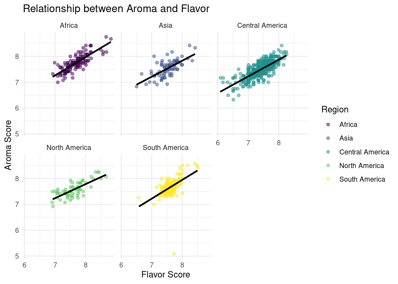
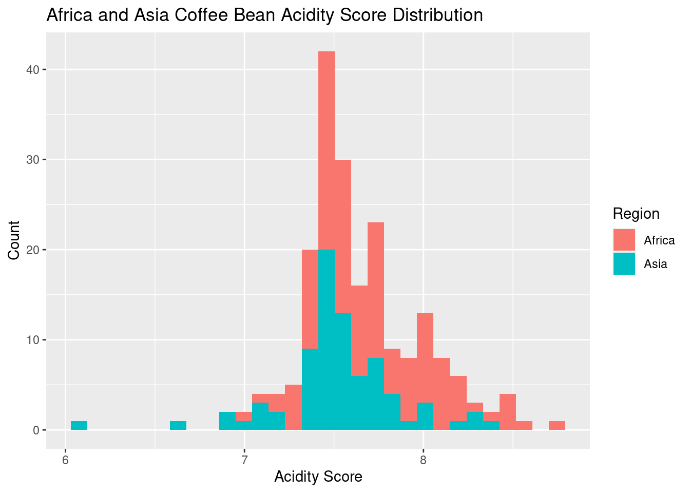
We imported a coffee dataset to answer the two following questions: how well does the flavor of coffee explain or predict how aromatic the beans will be and how does the acidity in coffee compare between beans grown in Africa versus those grown in Asia. Regarding the first question, we found a positive linear correlation between flavor and aroma. For the second, we found that coffee made from African beans tend to be slightly more acidic than those grown in Asia.
We wrangled the data in some ways to make it more applicable to our initial questions. We started by removing the columns we did not intend to use and changing some double types to numeric. We cleaned the variable names then proceeded to count the number of Arabica observations for each country. We created vectors for each region of countries and added a region column to each observation based on the vectors. We then counted the number of observations for each region and began visualizations with the wrangled data set.
Data description
This report uses data from the CORGIS Dataset Project by Sam Donald, created on July 6, 2020. It was originally curated by @jthomasmock in contribution to the Tidy Tuesday project on Github. The data contains observations that consist of two types of coffee beans (Arabica and Robusta) sampled from specific locations. There are 960 observations(rows). There are 16 attributes, or variables, that all specify information about the coffee bean that was sampled- the majority of them being a score. Such columns contain scores for things like the coffee’s acidity, sweetness, fragrance, etc. and are given a score from 1-10. There are also variables representing the average altitude of the location and the processing method of the beans.
The data was imported and cleaned for preprocessing by deleting columns not pertinent to the research topics, converting some double types to numeric, and cleaning the variable names. Based off the country of the observation, we sorted each observation into a different region. The different regions were: Africa, Asia, Central America, North America, and South America. Thus, we created a new column in the data called region that assigned the corresponding region to each observation after the dataset was filtered to only include Arabica beans. The project’s final dataset is called coffee_regions.
The information seen and recorded in this dataset may have been impacted by a number of mechanisms. The method used to collect the data, evaluators’ subjective rating, and potential prejudices against particular regions or coffee varieties, for example, could all have an impact on the results. It is reasonable to suppose that coffee professionals who evaluated and scored the beans according to their qualities contributed to the data gathering and that they would have anticipated that it would be used for research and analysis.
Data analysis
── Attaching packages ─────────────────────────────────────── tidyverse 1.3.2 ──
✔ ggplot2 3.4.0     ✔ purrr   1.0.0
✔ tibble  3.2.1     ✔ dplyr   1.1.2
✔ tidyr   1.2.1     ✔ stringr 1.5.0
✔ readr   2.1.3     ✔ forcats 0.5.2
── Conflicts ────────────────────────────────────────── tidyverse_conflicts() ──
✖ dplyr::filter() masks stats::filter()
✖ dplyr::lag()    masks stats::lag()

Attaching package: 'janitor'


The following objects are masked from 'package:stats':

    chisq.test, fisher.test


Attaching package: 'scales'


The following object is masked from 'package:purrr':

    discard


The following object is masked from 'package:readr':

    col_factor
Data summary
| Name |
coffee_regions2 |
| Number of rows |
960 |
| Number of columns |
3 |
| _______________________ |
|
| Column type frequency: |
|
| character |
1 |
| numeric |
2 |
| ________________________ |
|
| Group variables |
None |
Variable type: character
Variable type: numeric
| data_scores_aroma |
0 |
1 |
7.58 |
0.32 |
5.08 |
7.42 |
7.58 |
7.75 |
8.75 |
▁▁▂▇▁ |
| data_scores_flavor |
0 |
1 |
7.52 |
0.35 |
6.08 |
7.33 |
7.50 |
7.75 |
8.83 |
▁▂▇▃▁ |
── Attaching packages ────────────────────────────────────── tidymodels 1.0.0 ──
✔ broom        1.0.2     ✔ rsample      1.1.1
✔ dials        1.1.0     ✔ tune         1.1.1
✔ infer        1.0.4     ✔ workflows    1.1.2
✔ modeldata    1.0.1     ✔ workflowsets 1.0.0
✔ parsnip      1.0.3     ✔ yardstick    1.1.0
✔ recipes      1.0.6
── Conflicts ───────────────────────────────────────── tidymodels_conflicts() ──
✖ scales::discard() masks purrr::discard()
✖ dplyr::filter()   masks stats::filter()
✖ recipes::fixed()  masks stringr::fixed()
✖ dplyr::lag()      masks stats::lag()
✖ yardstick::spec() masks readr::spec()
✖ recipes::step()   masks stats::step()
• Learn how to get started at https://www.tidymodels.org/start/
Loading required package: airports
Loading required package: cherryblossom
Loading required package: usdata

Attaching package: 'openintro'

The following object is masked from 'package:modeldata':

    ames
# A tibble: 2 × 5
  term               estimate std.error statistic   p.value
  <chr>                 <dbl>     <dbl>     <dbl>     <dbl>
1 (Intercept)           2.53     0.149       17.0 9.30e- 57
2 data_scores_flavor    0.671    0.0198      33.9 4.29e-166
`geom_smooth()` using formula = 'y ~ x'
# A tibble: 1 × 12
  r.squared adj.r.squared sigma statistic   p.value    df logLik   AIC   BIC
      <dbl>         <dbl> <dbl>     <dbl>     <dbl> <dbl>  <dbl> <dbl> <dbl>
1     0.545         0.545 0.213     1148. 4.29e-166     1   125. -243. -228.
# ℹ 3 more variables: deviance <dbl>, df.residual <int>, nobs <int>
# A tibble: 1 × 1
  .pred
  <dbl>
1  7.90
# A tibble: 1 × 1
  mean_acid
      <dbl>
1      7.64
`stat_bin()` using `bins = 30`. Pick better value with `binwidth`.
Evaluation of significance
\[
\widehat{data~scores~aroma} = 2.53 + 0.67\times data~scores~flavor
\]
For each additional point of the flavor score, the predicted score of the aroma of the coffee beans is higher by 0.67 points, on average.
When the score flavor is 0, the aroma score is expected to be 2.53 points on average.
If we look at the R-squared and adjusted R-squared value of approximately 0.54, the percent variability in the response that is explained by our model appears to be 54%.
# A tibble: 1 × 2
  lower_ci upper_ci
     <dbl>    <dbl>
1    0.633    0.707
# A tibble: 2 × 5
  term               estimate std.error statistic   p.value
  <chr>                 <dbl>     <dbl>     <dbl>     <dbl>
1 (Intercept)          1.36     0.0204       66.6 0
2 data_scores_flavor   0.0887   0.00271      32.7 2.07e-158
We are 90% confident that the true aroma score is higher by 0.63 to 0.707 points for every additional flavor score point, on average.
\[
\log\Big(\frac{p}{1-p}\Big) = 1.357 + 0.089\times data~scores~flavor
\]
For each additional point of the flavor score, we expect the aroma score to be higher by 100 x [exp(0.089) -1], aka 9.31% points, on average.
When the score flavor is 0, the log odds of the aroma score is expected to be 1.357 points on average.
Response: data_scores_acidity (numeric)
Null Hypothesis: point
# A tibble: 1,000 × 2
   replicate  stat
       <int> <dbl>
 1         1 0.525
 2         2 0.464
 3         3 0.466
 4         4 0.536
 5         5 0.541
 6         6 0.525
 7         7 0.493
 8         8 0.477
 9         9 0.510
10        10 0.531
# ℹ 990 more rows
Bin width defaults to 1/30 of the range of the data. Pick better value with
`binwidth`.
Warning: Please be cautious in reporting a p-value of 0. This result is an
approximation based on the number of `reps` chosen in the `generate()` step. See
`?get_p_value()` for more information.
# A tibble: 1 × 1
  p_value
    <dbl>
1       0
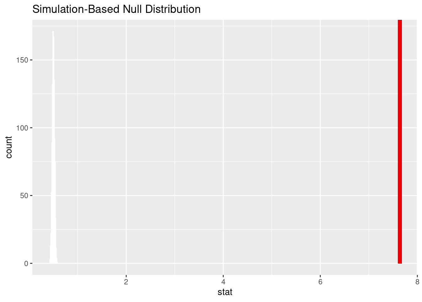
Null Hypothesis: There is no difference in the mean acidity score for the African and Asian regions.
\[
H_0: \mu_1 - \mu_2 = 0
\]
Alternative Hypothesis: There is a difference in the mean acidity score for the African and Asian regions.
\[
H_A: \mu_1 - \mu_2 \ne 0
\]
Given that the p value is 0 and that is less than the significance level of 0.05, we reject the null hypothesis in favor of the alternative hypothesis. The data provide convincing evidence that there is a difference in the mean acidity score for the African and Asian regions.
Interpretation and conclusions
For Analysis #1:
In data analysis 1, we investigated the relationship between the aroma and flavor scores of coffee beans. Our linear regression analysis demonstrated that for each additional point in the flavor score, the predicted score of the aroma of the coffee beans is higher by 0.67 points, on average. When the score flavor is 0, the aroma score is expected to be 2.53 points on average. Moreover, we conducted a bootstrapped hypothesis test and found that we are 90% confident that the true aroma score is higher by 0.63 to 0.707 points for every additional flavor score point, on average.
However, our R-squared value of 0.54 indicates that only 54% of the variability in the aroma score can be explained by the flavor score. Thus, we can not be completely confident in our model since a higher degree of correlation would probably be better. So, we then attempted to fit a logistic regression model to see if this fit the model better. We found that for each additional point of the flavor score, we expect the aroma score to be higher by 9.31% points, on average.
In the wider context of the real-life application, our findings indicate that there is a strong positive relationship between the flavor and aroma scores of coffee beans. This relationship can be beneficial for coffee farmers and traders because it establishes that focusing on improving the flavor profile of their beans can also lead to improvements in the aroma profile, which is an important aspect of coffee quality for many consumers. Furthermore, our findings can tell coffee tasters and judges in competitions, who often evaluate coffee aroma and flavor separately.
For Analysis #2:
In data analysis 2, we wanted to test whether there was a difference in the mean acidity score for the Africa versus Asia region. We discovered a difference of 0.17 between the mean acidity scores for the African and Asian regions, with the average for Africa being 7.71 points and the average for Asia being 7.54 points.
We performed a hypothesis test to see if this difference was significant. Our alternative hypothesis was that there was a difference between the two regions’ mean acidity scores, contrary to our null hypothesis that there was no difference. We utilized a bootstrap sampling method to get a null distribution of the mean acidity score difference and calculated the p-value of our observed mean difference.
The p-value was zero according to our analysis, which is less than our significance level of 0.05. As a result, we came to the conclusion that there is a significant difference in the mean acidity score between the African and Asian regions and rejected the null hypothesis while accepting the alternative hypothesis.
We can be confident in our conclusions because we utilized bootstrapping, which is a robust statistical method, and got a significant p-value. The coffee business, where the acidity score is a crucial aspect in establishing the quality of coffee beans, can benefit from these findings. For instance, when choosing which locations to get their beans from or how to sell their products to consumers, coffee producers and purchasers might take these distinctions into account.
Limitations
Firstly, one limitation of our project resides in the fact that the number of observations for each region is not equal. For example, the North America region contains 63 observations while Central America contains 494 observations. This has the potential of impacting our study when comparing coffee by region.
Another limitation is that we only calculated the acidity scores of coffee beans in Africa and Asia. In our future investigations, we can explore the acidity scores of all the other regions. This way we are able to explore if there is a relationship between acidity scores for each region. Thus, we can also explore the relationship of acidity scores to other factors or create an additive model to demonstrate if there are multiple factors affecting the acidity score of the coffee beans.
Overall, limitations also arise in the fact that bias could be introduced by the people scoring the coffee as scores could not be given out consistently if someone already has a pre harbored bias about coffee from a specific country or region.
Acknowledgments
We would like to express our gratitude to everyone who has supported this project.
First and foremost, we would like to thank Sam Donald for the data set that we were able to extrapolate our data from the CORGIS data set project. We would also like to to thank Tom Mock (@jthomasmock) in contribution to the Tidy Tuesday project on Github.
We are also grateful for the teaching assistants of this course for their office hours and for our project mentor in helping us choose a topic to begin with.
Our final project would not have been possible without these resources.