Analyzing Airbnb Data

Appendix to report

Appendix 1: Data cleaning

library(tidyverse)
library(skimr)
library(jsonlite)
library(dplyr)
library(scales)
library(tidymodels)
library(lubridate)
library(knitr)
library(kableExtra)
library(patchwork)
library(stringr)

theme_set(theme_minimal())
set.seed(123)

# Load airbnb listings data (03/06/2023)
airbnb_data <- read_csv("data/airbnb_data/03_06_2023_listings.csv", 
    col_types = cols(price = col_number()))

# Remove listings with price outliers
airbnb_data <- airbnb_data |> 
  filter(price < quantile(airbnb_data$price, 0.99))

# Load amenities dataframe from EDA
amenities <- read_csv("data/airbnb_data/amenities_data.csv")

Appendix 1A: Converting number of bathrooms from text to numeric

In our main dataset, the number of bathrooms is found in bathrooms_text and is presented as text instead of numeric. For example, you would see entries like “1 shared bath,” “2 baths,” and “2.5 baths.” This is quite troublesome for analysis. As such, we first extract the number in the entry. Them, we check any occurrence of the words “shared” and “private.” If the word “shared” is there, we divide the number by two.

listing <- airbnb_data %>%
  select(id, price, bedrooms, bathrooms_text) |> 
  drop_na(bathrooms_text)

listing$bathrooms <- str_extract(listing$bathrooms_text, "\\d+")

listing$bathrooms <- ifelse(str_detect(listing$bathrooms_text, "shared"), 
                                     as.numeric(listing$bathrooms)/2, 
                                     listing$bathrooms)

listing$bathrooms <- ifelse(str_detect(listing$bathrooms_text, "private"), 
                                     as.numeric(listing$bathrooms), 
                                     listing$bathrooms)

bathroom_tidy <- listing |>
  mutate(bathrooms = as.numeric(bathrooms))

write_csv(bathroom_tidy |> select(id, price, bathrooms), "data/airbnb_data/bathroom_tidy.csv")

Appendix 1B: Parsing through list of amenities

A major issue with amenities is that it is stored as a character list. We need to parse and clean this so that we can do more analysis.

amenities_df <- airbnb_data |>
  # Create subset of Airbnb data pertaining to amenities
  select(id, amenities) |>
  # Replace any occurrences of square brackets with empty string
  mutate(amenities = gsub("\\[|\\]", "", amenities)) |>
  # Split the list by comma and make separate rows
  separate_rows(amenities, sep = ", ") |>
  # Unnest the list
  unnest(amenities)

Appendix 1C: Identifying extra amenities

We wanted to conduct analysis on specific amenities, so we parsed out eight amenities that we consider as “extras:” air conditioning, heating, dishes and silverware, cooking basics, microwave, coffee maker, washer, and dryer.

extra_amenities <- c("air conditioning", "heating", "dishes and silverware", "cooking basics", "microwave", "coffee maker", "washer", "dryer")

extra_df <- data.frame(amenities) |> drop_na(amenities)
  
for (amenity in extra_amenities) {
  extra_df <- extra_df |>
    mutate(!!amenity :=
      str_detect(
        extra_df$amenities,
        regex(amenity, ignore_case = TRUE)
      ))
}

extra_df <- extra_df |>
  group_by(id) |>
  summarise(
    air_conditioning = any(`air conditioning`),
    heating = any(heating),
    dishes_and_silverware = any(`dishes and silverware`),
    cooking_basics = any(`cooking basics`),
    microwave = any(microwave),
    coffee_maker = any(`coffee maker`),
    washer = any(washer),
    dryer = any(dryer)
  )

extra_all <- extra_df |> 
  mutate(
    all_extras = 
      air_conditioning &
      heating &
      dishes_and_silverware &
      cooking_basics&microwave &
      coffee_maker &
      washer &
      dryer
  ) |> merge(airbnb_data |> select(id, price))

write.csv(extra_all, "data/airbnb_data/extra_amenities.csv", row.names=FALSE)

Appendix 1D: Identifying work-from-home amenities

Similar to our extra amenities analysis, we decided to look into how work-from-home (WFH) amenities play a role in affecting price, and whether or not it can be a good price predictor. We decided to look into three WFH criteria:

The listing must offer Wifi, which we determined by checking its list of amenities.
The listing must offer a dedicated workspace, which we determined by checking its list of amenities.
The listing must be located in a quiet environment. To determine this, we searched for occurrences of the word “quiet” in the listing’s name and description.

wfh_amenities <- data.frame(amenities) |> drop_na(amenities)

for (amenity in c("wifi", "workspace")) {
  wfh_amenities <- wfh_amenities |>
    mutate(!!amenity :=
      str_detect(
        wfh_amenities$amenities,
        regex(amenity, ignore_case = TRUE)
      ))
}

wfh_amenities <- wfh_amenities |>
  group_by(id) |>
  summarise(
    wifi = any(wifi),
    workspace = any(workspace)
  )

listings_with_quiet <- airbnb_data |> 
  select(id) |> 
  mutate(
    quiet = case_when(
      str_detect(airbnb_data$name, regex("quiet", ignore_case = TRUE)) ~ TRUE,
      str_detect(airbnb_data$description, regex("quiet", ignore_case = TRUE)) ~ TRUE
      ,TRUE ~ FALSE
    )
  )

wifi_work_quiet <- merge(wfh_amenities, listings_with_quiet) |> 
  mutate(
    all_three = wifi&workspace&quiet,
    wifi_workspace_only = wifi&workspace&(!quiet),
    wifi_only =  wifi&(!workspace)&(!quiet)
  ) |> 
  merge(airbnb_data |> select(id, neighbourhood_cleansed, 
                              neighbourhood_group_cleansed, price)) |> 
  drop_na()

write.csv(wifi_work_quiet, "data/airbnb_data/wfh_amenities.csv", row.names=FALSE)

Appendix 1E: Cleaning up host characteristics

To see how host characteristics vary, we need to make sure that the hosts with multiple listings are only displayed once. To do this, we only include unique host IDs. By doing so, the price and various review scores only display the values associated with whichever listing remains. To avoid this, we average these values by grouping the host IDs. The following analysis is built on these averaged prices and host characteristics.

host <- airbnb_data |>
  select(
    host_id,
    host_is_superhost,
    host_identity_verified,
    review_scores_cleanliness,
    review_scores_communication,
    host_response_time,
    host_acceptance_rate,
    price,
  ) |>
  drop_na() |>
  group_by(host_id) |>
  mutate(price = mean(price)) |>
  distinct(host_id, .keep_all = TRUE) |>
  mutate(price = log(price)) |>
  ungroup()

# Superhost dataframe
superhosts <- host |>
  select(host_is_superhost) |>
  mutate(host_is_superhost = if_else(host_is_superhost == TRUE, "Superhost", "Not superhost")) |>
  count(host_is_superhost)

# Superhost visual
superhost_graph <-
  ggplot(host, mapping = aes(x = host_is_superhost)) +
  geom_bar() +
  theme_minimal() +
  scale_x_discrete(limits = rev,
                   labels = c("Superhost", "Not superhost")) +
  labs(title = "# of superhosts",
       x = "",
       y = "Count")

# Host identity verified dataframe
identity_verified <- host |>
  select(host_identity_verified) |>
  mutate(host_identity_verified = if_else(host_identity_verified == TRUE, "Verified", "Not verified")) |>
  count(host_identity_verified)

# Host identity verified graph
identity_verified_graph <-
  ggplot(host, mapping = aes(x = host_identity_verified)) +
  geom_bar() +
  theme_minimal() +
  scale_x_discrete(limits = rev,
                   labels = c("Verified", "Not verified")) +
  labs(title = "# of verified hosts",
       x = "",
       y = "")

# Review score cleanliness dataframe
cleanliness <- host |>
  select(review_scores_cleanliness) |>
  mutate(
    scores = case_when(
      4 < review_scores_cleanliness &
        review_scores_cleanliness <= 5 ~ "Very high",
      3 < review_scores_cleanliness &
        review_scores_cleanliness <= 4 ~ "High",
      2 < review_scores_cleanliness &
        review_scores_cleanliness <= 3 ~ "Medium",
      1 < review_scores_cleanliness &
        review_scores_cleanliness <= 2 ~ "Low",
      review_scores_cleanliness <= 1 ~ "Very low",
    ),
    cleanliness_score = fct_relevel(scores, "Very low", "Low", "Medium", "High", "Very high")
  ) |>
  count(cleanliness_score)

# Review score cleanliness graph
cleanliness_graph <- ggplot(cleanliness, mapping = aes(x = cleanliness_score, y = n)) +
  geom_col() +
  theme_minimal() +
  labs(title = "Host cleanliness rating",
       x = "",
       y = "")

# Review score communication dataframe
communication <- host |>
  select(review_scores_communication) |>
  mutate(
    scores = case_when(
      4 < review_scores_communication &
        review_scores_communication <= 5 ~ "Very high",
      3 < review_scores_communication &
        review_scores_communication <= 4 ~ "High",
      2 < review_scores_communication &
        review_scores_communication <= 3 ~ "Medium",
      1 < review_scores_communication &
        review_scores_communication <= 2 ~ "Low",
      review_scores_communication <= 1 ~ "Very low",
    ),
    communication_score = fct_relevel(scores, "Very low", "Low", "Medium", "High", "Very high")
  ) |>
  count(communication_score)

# Review score communication graph
communication_graph <-
  ggplot(communication, mapping = aes(x = communication_score, y = n)) +
  geom_col() +
  theme_minimal() +
  labs(title = "Host communication rating",
       x = "",
       y = "")

# Host response time dataframe
response <- host |>
  select(host_response_time, price) |>
  count(host_response_time) |>
  mutate(
    Time = fct_relevel(
      host_response_time,
      "within an hour",
      "within a few hours",
      "within a day",
      "a few days or more"
    )
  )

response[response == "N/A"]  <- NA

response <- na.omit(response)

# Host response time graph
response_time_graph <-
  ggplot(response, mapping = aes(x = host_response_time, y = n)) +
  geom_col() +
  scale_x_discrete(
    limits = rev,
    labels = c(
      "within an hour",
      "within a few hours",
      "within a day",
      "a few days or more"
    )
  ) +
  theme_minimal() +
  labs(title = "Hosts by their response time",
       x = "",
       y = "Count")

# Host acceptance rate dataframe
acceptance <- host |>
  select(host_acceptance_rate)

acceptance[acceptance == "N/A"]  <- NA

acceptance <- na.omit(acceptance)

acceptance <- acceptance |>
  mutate(
    host_acceptance_rate = substr(host_acceptance_rate, 1, nchar(host_acceptance_rate)-1),
    host_acceptance_rate = as.numeric(host_acceptance_rate)) |>
  count(host_acceptance_rate)

# Host acceptance rate graph
acceptance_graph <-
  ggplot(acceptance, mapping = aes(x = host_acceptance_rate, y = n)) +
  geom_col() +
  theme_minimal() +
  labs(title = "Hosts by their acceptance rate",
       x = "",
       y = "Count")

Appendix 1F: Model fitting and evaluation

We created main_variable_dataset to have a centralized dataset to conduct our multivariate linear regression analysis and other ML model fitting.

main_variable_dataset <- wifi_work_quiet |> 
  select(id, wifi, workspace, quiet) |> 
  merge(extra_all |> 
          select(id, air_conditioning, heating, dishes_and_silverware, 
                 cooking_basics, microwave, coffee_maker, washer, dryer, price)) |> 
  merge(bathroom_tidy |> select(id, bathrooms)) |> 
  merge(airbnb_data |> select(id, neighbourhood_group_cleansed,
                              bedrooms, room_type, 
                              host_is_superhost, 
                              host_identity_verified,
                              review_scores_cleanliness,
                              review_scores_communication,
                              review_scores_rating,
                              host_response_time,
                              host_acceptance_rate)) 

main_variable_dataset[main_variable_dataset == "N/A"]  <- NA

main_variable_dataset <- na.omit(main_variable_dataset)

main_variable_dataset <- main_variable_dataset |>
  mutate(
    host_acceptance_rate = substr(host_acceptance_rate, 1, nchar(host_acceptance_rate)-1),
    host_acceptance_rate = as.numeric(host_acceptance_rate)
  )
write_csv(main_variable_dataset, "data/airbnb_data/main_variable_dataset.csv")

Appendix 2: Additional analyses

Appendix 2A: Bathroom-to-bedroom ratio

The bathroom-to-bedroom ratio is an interesting factor in determining the price of Airbnb. Usually, luxury stayings tend to have a higher bathroom-to-bedroom ratio, which means there are more bathrooms than bedrooms. We will check if the assumption is true.

# Create a new variable for bathroom-to-bedroom ratio
ratio_listing <- mutate(bathroom_tidy, bath_bed_ratio = as.numeric(bathrooms) / bedrooms)

ratio_listing

# A tibble: 42,426 × 6
        id price bedrooms bathrooms_text bathrooms bath_bed_ratio
     <dbl> <dbl>    <dbl> <chr>              <dbl>          <dbl>
 1 8.02e17   143        1 1 bath               1            1    
 2 7.66e17    30        1 1 shared bath        0.5          0.5  
 3 6.36e17   157        2 2 baths              2            1    
 4 7.68e17    89        3 2 baths              2            0.667
 5 4.92e 7   125        2 1 bath               1            0.5  
 6 5.21e 7    63        1 1 shared bath        0.5          0.5  
 7 7.83e17    82        1 1 shared bath        0.5          0.5  
 8 3.91e 7   118        1 1 bath               1            1    
 9 6.55e17    49        1 1 shared bath        0.5          0.5  
10 6.73e 6   115        2 1 bath               1            0.5  
# ℹ 42,416 more rows

# Create a histogram to visualize the distribution
ratio_listing |>
  ggplot(aes(x = bath_bed_ratio)) +
  geom_histogram(binwidth = 0.5, fill = "#008FD5", color = "black") +
  labs(title = "Bathroom-to-bedroom Ratio Distribution",
       x = "Bathroom-to-bedroom Ratio",
       y = "Frequency")

Warning: Removed 3858 rows containing non-finite values (`stat_bin()`).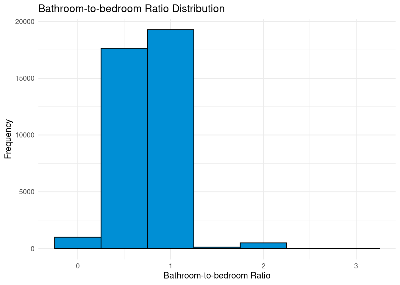

ratio_listing |>
  filter(bath_bed_ratio %in% c(1,2,3,4)) |> 
  ggplot(aes(x = bath_bed_ratio, y = price)) +
  geom_boxplot() +
  facet_wrap(vars(bath_bed_ratio)) +
  scale_y_continuous(limits = quantile(listing$price, c(0, 0.9))) +
  labs(x = "Bathroom-to-bedroom ratio",
       y = "Price",
       title = "Price vs. Bathroom-to-bedroom ratio on Airbnb in NYC")+
  theme(axis.text.x = element_blank())

Warning: Continuous x aesthetic
ℹ did you forget `aes(group = ...)`?

Warning: Removed 2308 rows containing non-finite values (`stat_boxplot()`).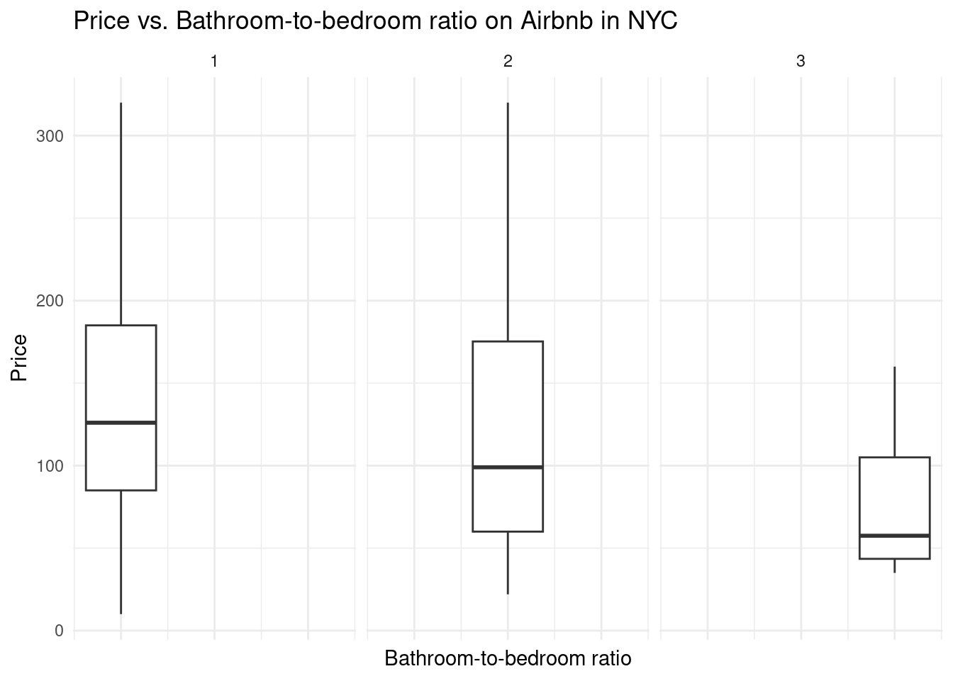

logprice_ratio_fit <- linear_reg() |>
  fit(log(price) ~ bath_bed_ratio, data = ratio_listing)

Appendix 2B: Proportion of listings with extra amenities and price difference

extra_all_neighbourhood <-
  merge(extra_all, airbnb_data |>
          select(id, price,
                 neighbourhood_group_cleansed, neighbourhood_cleansed)) |>
  select(id, all_extras, price,
         neighbourhood_group_cleansed, neighbourhood_cleansed) |>
  drop_na()

extra_all_borough_table <- extra_all_neighbourhood |>
  group_by(neighbourhood_group_cleansed) |>
  summarize(
    count = n(),
    prop_all_extras = signif(sum(all_extras)/n(), 3)
  ) |>
  arrange(desc(prop_all_extras)) |>
  set_names(c("Borough", "Number of listings", "Proportion of listings with all extra amenities included"))

kable(extra_all_borough_table,
      caption = "Proportion of listings with all extra amenities included by borough",
             align = "l") |> 
  kable_classic()

Proportion of listings with all extra amenities included by borough
Borough	Number of listings	Proportion of listings with all extra amenities included
Staten Island	426	0.1850
Manhattan	17219	0.1400
Brooklyn	16094	0.1390
Bronx	1680	0.0857
Queens	6885	0.0840

extra_table <- extra_all_neighbourhood |> 
  mutate(
    all_extras = factor(ifelse(all_extras, "Yes", "No"))
  ) |> 
  group_by(all_extras) |> 
  summarise(
    median_price = signif(median(price), 3)
  )  |> 
  arrange(desc(median_price)) |> 
  mutate(
    median_price = dollar(median_price)
  )  |> 
  set_names(c("Does the listing have all the extras?", "Median price"))

kable(extra_table, 
             align = "l") |> 
  kable_classic()

Does the listing have all the extras?	Median price
Yes	$175
No	$120

Appendix 2C: Additive and interactive linear regressions with respect to extra amenities

Below, we fit additive and interactive linear regression models for extra amenities. As expected, we see that the interactive model produced a higher R-squared value than the additive model. Moreover, we see that both models produced R-squared values of above 10%, which suggests that extra amenities are not negligible in affecting price.

linear_all_interactive <- linear_reg() |>
  fit(log(price) ~
        air_conditioning * heating * dishes_and_silverware * 
        cooking_basics * microwave * coffee_maker * washer * dryer, 
      data = extra_all |> drop_na() |> filter(price != 0))

linear_all_additive <- linear_reg() |>
  fit(log(price) ~ air_conditioning + heating + dishes_and_silverware + 
        cooking_basics + microwave + coffee_maker + washer + dryer,
      data = extra_all |> drop_na() |> filter(price != 0))

kable(
  glance(linear_all_interactive),
  caption = 
    "Interactive Linear Regression of log(price) with respect to extra amenities",
  align = "l") |>
  kable_classic()

Interactive Linear Regression of log(price) with respect to extra amenities
r.squared	adj.r.squared	sigma	statistic	p.value	df	logLik	AIC	BIC	deviance	df.residual	nobs
0.1748675	0.1700972	0.6607168	36.65805	0	243	-42345.26	85180.51	87300.25	18349.37	42033	42277

kable(
  glance(linear_all_additive),
  caption = 
    "Additive Linear Regression of log(price) with respect to extra amenities",
  align = "l") |>
  kable_classic()

Additive Linear Regression of log(price) with respect to extra amenities
r.squared	adj.r.squared	sigma	statistic	p.value	df	logLik	AIC	BIC	deviance	df.residual	nobs
0.1164623	0.116295	0.6817975	696.4369	0	8	-43790.92	87601.84	87688.36	19648.19	42268	42277

Appendix 2D: Proportion of listings with WFH amenities and price difference

wfh_final_borough_table <- wifi_work_quiet |> 
  group_by(neighbourhood_group_cleansed) |> 
  summarize(
    count = n(),
    prop_all_three = signif(sum(all_three)/n(), 3),
    prop_wifi_workspace_only = signif(sum(wifi_workspace_only)/n(), 3),
    prop_wifi_only = signif(sum(wifi_only)/n(), 3)
  ) |> 
  arrange(desc(prop_all_three)) |> 
  set_names(c("Borough", "Number of listings", "Proportion of listings with all three criteria met", "Proportion of listings with Wifi and workspace only", "Proportion of listings with Wifi only"))

kable(wfh_final_borough_table, 
      caption = "Proportion of listings with WFH criteria satisfied by borough",
             align = "l") |> 
  kable_classic()

Proportion of listings with WFH criteria satisfied by borough
Borough	Number of listings	Proportion of listings with all three criteria met	Proportion of listings with Wifi and workspace only	Proportion of listings with Wifi only
Staten Island	426	0.1380	0.354	0.366
Bronx	1680	0.1110	0.367	0.382
Queens	6885	0.0959	0.377	0.411
Brooklyn	16094	0.0857	0.337	0.446
Manhattan	17219	0.0638	0.313	0.496

wfh_table <- wifi_work_quiet |> 
  mutate(
    all_three = factor(ifelse(all_three, "Yes", "No"))
  ) |> 
  group_by(all_three) |> 
  summarise(
    median_price = signif(median(price), 3)
  )  |> 
  arrange(desc(median_price)) |> 
  mutate(
    median_price = dollar(median_price)
  ) |> 
  set_names(c("Does the listing satisfy all WFH criteria?", "Median price"))

kable(wfh_table, 
             align = "l") |> 
  kable_classic()

Does the listing satisfy all WFH criteria?	Median price
Yes	$130
No	$124

Appendix 2E: Additive and interactive linear regressions with respect to work-from-home amenities

Below, we fit additive and interactive linear regression models for WFH amenities. The two models produced similar R-squared values, which suggests that WFH amenities are negligible in affecting price.

wfh_interactive <- linear_reg() |>
  fit(log(price) ~
        wifi * workspace * quiet, 
      data = wifi_work_quiet |> filter(price != 0))

wfh_additive <- linear_reg() |>
  fit(log(price) ~
        wifi + workspace + quiet,
      data = wifi_work_quiet |> filter(price != 0))

kable(
  glance(wfh_interactive),
  caption = 
    "Interactive Linear Regression of log(price) with respect to WFH criteria",
  align = "l") |>
  kable_classic()

Interactive Linear Regression of log(price) with respect to WFH criteria
r.squared	adj.r.squared	sigma	statistic	p.value	df	logLik	AIC	BIC	deviance	df.residual	nobs
0.0159578	0.0157948	0.7195228	97.92261	0	7	-46068.27	92154.54	92232.41	21883.22	42269	42277

kable(
  glance(wfh_additive),
  caption = 
    "Additive Linear Regression of log(price) with respect to WFH criteria",
  align = "l") |>
  kable_classic()

Additive Linear Regression of log(price) with respect to WFH criteria
r.squared	adj.r.squared	sigma	statistic	p.value	df	logLik	AIC	BIC	deviance	df.residual	nobs
0.0159044	0.0158346	0.7195083	227.7314	0	3	-46069.42	92148.83	92192.09	21884.4	42273	42277

Appendix 2F: Trends of host characteristics

superhost_graph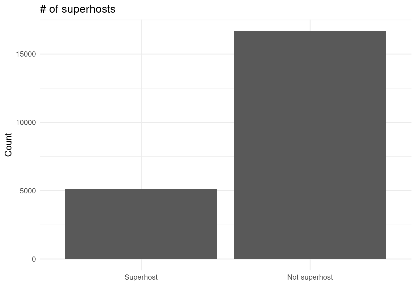

identity_verified_graph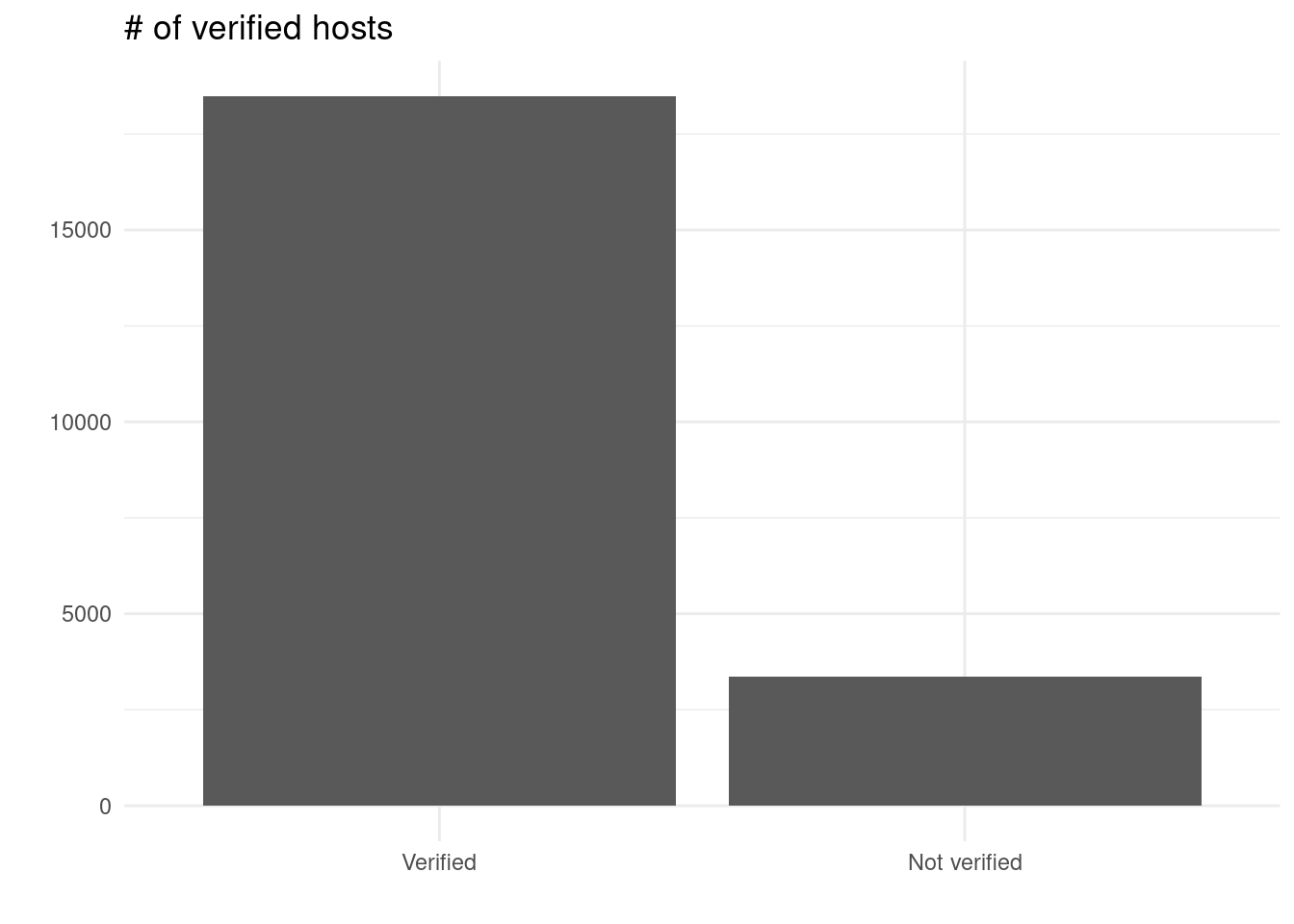

cleanliness_graph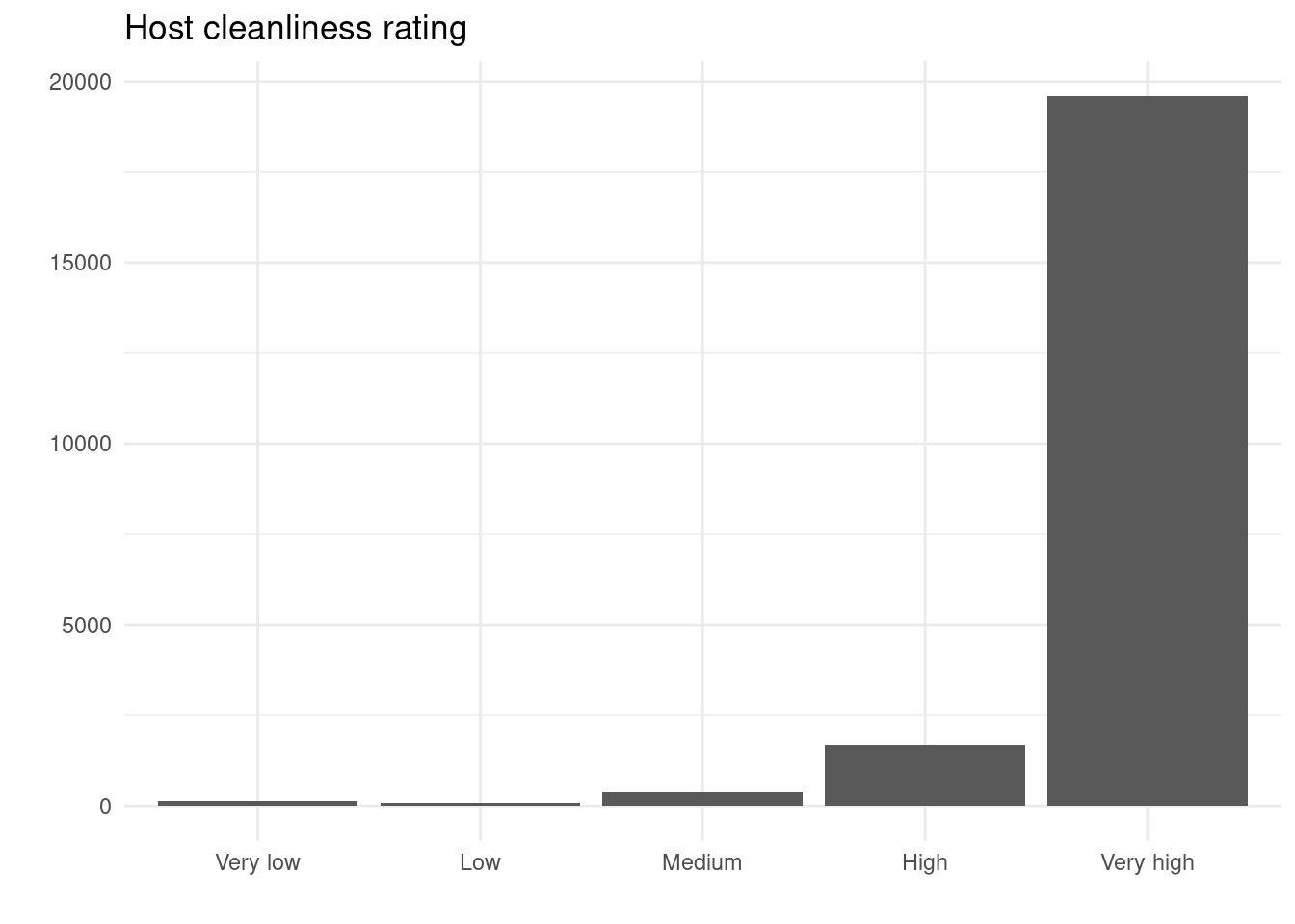

communication_graph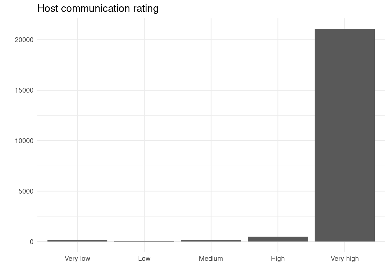

response_time_graph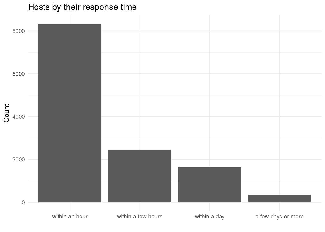

acceptance_graph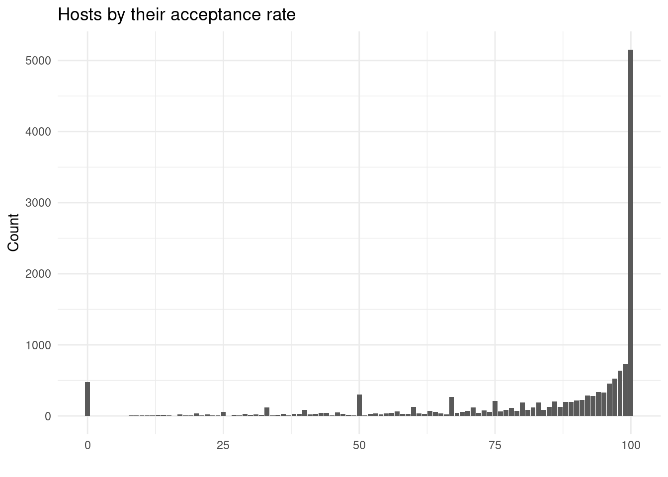

superhosts_perc <-
  tibble(perc = superhosts$n[2] / sum(superhosts$n) * 100)

identity_verified_perc <-
  tibble(perc = identity_verified$n[2] / sum(identity_verified$n) * 100)

cleanliness_perc <- cleanliness |>
  mutate(perc = n / sum(n) * 100) |>
  select(cleanliness_score, perc)

communication_perc <- communication |>
  mutate(perc = n / sum(n) * 100) |>
  select(communication_score, perc)

response_perc <- response |>
  mutate(Percent = n / sum(n) * 100) |>
  select(Time, Percent)

acceptance <- host |>
  select(host_acceptance_rate)

acceptance[acceptance == "N/A"]  <- NA

acceptance <- na.omit(acceptance)

acceptance <- acceptance |>
  mutate(
    host_acceptance_rate = substr(host_acceptance_rate, 1, nchar(host_acceptance_rate)-1),
    host_acceptance_rate = as.numeric(host_acceptance_rate))

acceptance_perc <-
  tibble(perc = mean(acceptance$host_acceptance_rate))

host_char_percs_1 <- tribble(
  ~ `Host characteristic`, ~ `Percent`,
  "Superhost", superhosts_perc$perc,
  "Identity is verified", identity_verified_perc$perc,
  "Host acceptance rate", acceptance_perc$perc,
) |> 
  arrange(desc(`Percent`))

host_char_percs_2 <- tribble(
  ~ `Rating`, ~ `Cleanliness review`, ~ `Communication review`,
  cleanliness_perc$cleanliness_score[1], cleanliness_perc$perc[1], communication_perc$perc[1],
  cleanliness_perc$cleanliness_score[2], cleanliness_perc$perc[2], communication_perc$perc[2],
  cleanliness_perc$cleanliness_score[3], cleanliness_perc$perc[3], communication_perc$perc[3],
  cleanliness_perc$cleanliness_score[4], cleanliness_perc$perc[4], communication_perc$perc[4],
  cleanliness_perc$cleanliness_score[5], cleanliness_perc$perc[5], communication_perc$perc[5],
)

kable(host_char_percs_1, 
             caption = "Trends of host characteristics",
             align = "l") |> 
  kable_classic()

Trends of host characteristics
Host characteristic	Percent
Identity is verified	84.65167
Host acceptance rate	84.10369
Superhost	23.54234

kable(host_char_percs_2, 
             caption = "Trends of host reviews",
             align = "l") |> 
  kable_classic()

Trends of host reviews
Rating	Cleanliness review	Communication review
Very low	0.6000092	0.4763432
Low	0.3480969	0.1374067
Medium	1.6763615	0.5542069
High	7.6352311	2.2809509
Very high	89.7403014	96.5510924

kable(response_perc, 
             caption = "Host response rate",
             align = "l") |> 
  kable_classic()

Host response rate
Time	Percent
a few days or more	2.61817
within a day	13.08301
within a few hours	19.07972
within an hour	65.21910

Appendix 2G: Acceptance rate hypothesis testing

accept <- host |>
  select(host_acceptance_rate, price) |>
  mutate(host_acceptance_rate = if_else(
    0 <= host_acceptance_rate & host_acceptance_rate < 51, TRUE, FALSE
  ))

point_diff_acceptance <- accept |>
  specify(price ~ host_acceptance_rate) |>
  calculate(stat = "diff in medians", order = c(TRUE, FALSE))

null_dist_acceptance <- accept |>
  specify(price ~ host_acceptance_rate) |>
  hypothesize(null = "independence") |>
  generate(reps = 1000, type = "permute") |>
  calculate(stat = "diff in medians", order = c(TRUE, FALSE))

visualize(null_dist_acceptance) +
  shade_p_value(obs_stat = point_diff_acceptance, direction = "greater")

Warning in min(diff(unique_loc)): no non-missing arguments to min; returning Inf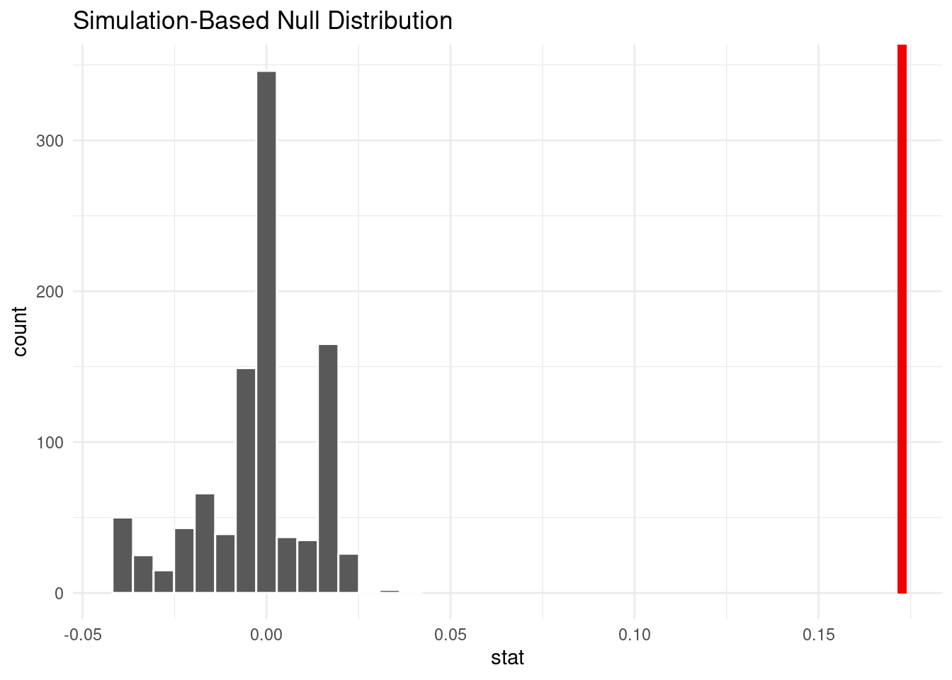

get_p_value(null_dist_acceptance,
            obs_stat = point_diff_acceptance,
            direction = "greater")

Warning: Please be cautious in reporting a p-value of 0. This result is an
approximation based on the number of `reps` chosen in the `generate()` step. See
`?get_p_value()` for more information.

# A tibble: 1 × 1
  p_value
    <dbl>
1       0

Appendix 2H: Cleanliness score hypothesis testing

clean <- host |>
  select(review_scores_cleanliness, price) |>
  mutate(review_scores_cleanliness = if_else(
    4.0 < review_scores_cleanliness & review_scores_cleanliness <= 5.0, TRUE, FALSE
  ))

point_diff_cleanliness <- clean |>
  specify(price ~ review_scores_cleanliness) |>
  calculate(stat = "diff in medians", order = c(TRUE, FALSE))

null_dist_cleanliness <- clean |>
  specify(price ~ review_scores_cleanliness) |>
  hypothesize(null = "independence") |>
  generate(reps = 1000, type = "permute") |>
  calculate(stat = "diff in medians", order = c(TRUE, FALSE))

visualize(null_dist_cleanliness) +
  shade_p_value(obs_stat = point_diff_cleanliness, direction = "greater")

Warning in min(diff(unique_loc)): no non-missing arguments to min; returning Inf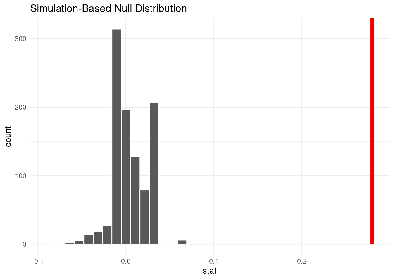

get_p_value(null_dist_cleanliness,
            obs_stat = point_diff_cleanliness,
            direction = "greater")

Warning: Please be cautious in reporting a p-value of 0. This result is an
approximation based on the number of `reps` chosen in the `generate()` step. See
`?get_p_value()` for more information.

# A tibble: 1 × 1
  p_value
    <dbl>
1       0

Appendix 2I: Backward elimination to isolate significant predictors

We performed backward elimination on our full multivariate linear regression model to come up with a list of significant predictors.

# remove overall rating
all_21_fit <- linear_reg() |>
  fit(log(price) ~ neighbourhood_group_cleansed + 
        wifi +
        workspace +
        quiet +
        host_is_superhost +
        host_identity_verified +
        review_scores_cleanliness +
        review_scores_communication +
        # review_scores_rating +
        host_response_time +
        host_acceptance_rate +
        air_conditioning +
        heating +
        dishes_and_silverware +
        cooking_basics +
        microwave +
        coffee_maker +
        washer +
        dryer +
        room_type +
        bedrooms +
        bathrooms,
      data = main_variable_dataset)
glance(all_21_fit)

# A tibble: 1 × 12
  r.squared adj.r.squared sigma statistic p.value    df  logLik    AIC    BIC
      <dbl>         <dbl> <dbl>     <dbl>   <dbl> <dbl>   <dbl>  <dbl>  <dbl>
1     0.608         0.608 0.433     1102.       0    28 -11545. 23150. 23387.
# ℹ 3 more variables: deviance <dbl>, df.residual <int>, nobs <int>

tidy(all_21_fit)

# A tibble: 29 × 5
   term                                   estimate std.error statistic   p.value
   <chr>                                     <dbl>     <dbl>     <dbl>     <dbl>
 1 (Intercept)                              3.83     0.0576      66.5  0        
 2 neighbourhood_group_cleansedBrooklyn     0.177    0.0142      12.5  1.76e- 35
 3 neighbourhood_group_cleansedManhattan    0.503    0.0145      34.6  6.62e-255
 4 neighbourhood_group_cleansedQueens       0.0571   0.0149       3.84 1.25e-  4
 5 neighbourhood_group_cleansedStaten Is…  -0.0430   0.0283      -1.52 1.28e-  1
 6 wifiTRUE                                -0.122    0.0344      -3.55 3.85e-  4
 7 workspaceTRUE                            0.0460   0.00642      7.17 7.90e- 13
 8 quietTRUE                               -0.0388   0.00764     -5.08 3.74e-  7
 9 host_is_superhostTRUE                    0.0277   0.00685      4.05 5.24e-  5
10 host_identity_verifiedTRUE               0.0256   0.00941      2.72 6.60e-  3
# ℹ 19 more rows

# remove communcation rating
all_20_fit <- linear_reg() |>
  fit(log(price) ~ neighbourhood_group_cleansed + 
        wifi +
        workspace +
        quiet +
        host_is_superhost +
        host_identity_verified +
        review_scores_cleanliness +
        # review_scores_communication +
        # review_scores_rating +
        host_response_time +
        host_acceptance_rate +
        air_conditioning +
        heating +
        dishes_and_silverware +
        cooking_basics +
        microwave +
        coffee_maker +
        washer +
        dryer +
        room_type +
        bedrooms +
        bathrooms,
      data = main_variable_dataset)
glance(all_20_fit)

# A tibble: 1 × 12
  r.squared adj.r.squared sigma statistic p.value    df  logLik    AIC    BIC
      <dbl>         <dbl> <dbl>     <dbl>   <dbl> <dbl>   <dbl>  <dbl>  <dbl>
1     0.608         0.608 0.433     1142.       0    27 -11546. 23151. 23380.
# ℹ 3 more variables: deviance <dbl>, df.residual <int>, nobs <int>

tidy(all_20_fit)

# A tibble: 28 × 5
   term                                   estimate std.error statistic   p.value
   <chr>                                     <dbl>     <dbl>     <dbl>     <dbl>
 1 (Intercept)                              3.79     0.0533      71.1  0        
 2 neighbourhood_group_cleansedBrooklyn     0.176    0.0142      12.4  2.99e- 35
 3 neighbourhood_group_cleansedManhattan    0.502    0.0145      34.6  1.47e-254
 4 neighbourhood_group_cleansedQueens       0.0569   0.0149       3.82 1.33e-  4
 5 neighbourhood_group_cleansedStaten Is…  -0.0437   0.0283      -1.54 1.23e-  1
 6 wifiTRUE                                -0.123    0.0344      -3.59 3.32e-  4
 7 workspaceTRUE                            0.0459   0.00642      7.15 9.15e- 13
 8 quietTRUE                               -0.0392   0.00763     -5.14 2.78e-  7
 9 host_is_superhostTRUE                    0.0272   0.00684      3.98 6.98e-  5
10 host_identity_verifiedTRUE               0.0256   0.00941      2.72 6.44e-  3
# ℹ 18 more rows

# remove identity verify

all_19_fit <- linear_reg() |>
  fit(log(price) ~ neighbourhood_group_cleansed + 
        wifi +
        workspace +
        quiet +
        host_is_superhost +
        # host_identity_verified +
        review_scores_cleanliness +
        # review_scores_communication +
        # review_scores_rating +
        host_response_time +
        host_acceptance_rate +
        air_conditioning +
        heating +
        dishes_and_silverware +
        cooking_basics +
        microwave +
        coffee_maker +
        washer +
        dryer +
        room_type +
        bedrooms +
        bathrooms,
      data = main_variable_dataset)
glance(all_19_fit)

# A tibble: 1 × 12
  r.squared adj.r.squared sigma statistic p.value    df  logLik    AIC    BIC
      <dbl>         <dbl> <dbl>     <dbl>   <dbl> <dbl>   <dbl>  <dbl>  <dbl>
1     0.608         0.607 0.433     1185.       0    26 -11550. 23156. 23378.
# ℹ 3 more variables: deviance <dbl>, df.residual <int>, nobs <int>

tidy(all_19_fit)

# A tibble: 27 × 5
   term                                   estimate std.error statistic   p.value
   <chr>                                     <dbl>     <dbl>     <dbl>     <dbl>
 1 (Intercept)                              3.81     0.0529      72.0  0        
 2 neighbourhood_group_cleansedBrooklyn     0.178    0.0142      12.5  8.16e- 36
 3 neighbourhood_group_cleansedManhattan    0.505    0.0145      34.8  2.08e-257
 4 neighbourhood_group_cleansedQueens       0.0578   0.0149       3.89 1.02e-  4
 5 neighbourhood_group_cleansedStaten Is…  -0.0464   0.0283      -1.64 1.01e-  1
 6 wifiTRUE                                -0.120    0.0344      -3.50 4.65e-  4
 7 workspaceTRUE                            0.0465   0.00642      7.24 4.49e- 13
 8 quietTRUE                               -0.0394   0.00763     -5.17 2.41e-  7
 9 host_is_superhostTRUE                    0.0270   0.00684      3.94 8.19e-  5
10 review_scores_cleanliness                0.123    0.00670     18.3  3.66e- 74
# ℹ 17 more rows

# review dishes and silverware
all_18_fit <- linear_reg() |>
  fit(log(price) ~ neighbourhood_group_cleansed + 
        wifi +
        workspace +
        quiet +
        host_is_superhost +
        # host_identity_verified +
        review_scores_cleanliness +
        # review_scores_communication +
        # review_scores_rating +
        host_response_time +
        host_acceptance_rate +
        air_conditioning +
        heating +
        # dishes_and_silverware +
        cooking_basics +
        microwave +
        coffee_maker +
        washer +
        dryer +
        room_type +
        bedrooms +
        bathrooms,
      data = main_variable_dataset)
glance(all_18_fit)

# A tibble: 1 × 12
  r.squared adj.r.squared sigma statistic p.value    df  logLik    AIC    BIC
      <dbl>         <dbl> <dbl>     <dbl>   <dbl> <dbl>   <dbl>  <dbl>  <dbl>
1     0.608         0.607 0.433     1232.       0    25 -11556. 23165. 23378.
# ℹ 3 more variables: deviance <dbl>, df.residual <int>, nobs <int>

tidy(all_18_fit)

# A tibble: 26 × 5
   term                                   estimate std.error statistic   p.value
   <chr>                                     <dbl>     <dbl>     <dbl>     <dbl>
 1 (Intercept)                              3.81     0.0529      72.0  0        
 2 neighbourhood_group_cleansedBrooklyn     0.177    0.0142      12.5  1.31e- 35
 3 neighbourhood_group_cleansedManhattan    0.505    0.0145      34.8  1.64e-257
 4 neighbourhood_group_cleansedQueens       0.0577   0.0149       3.87 1.07e-  4
 5 neighbourhood_group_cleansedStaten Is…  -0.0454   0.0283      -1.61 1.08e-  1
 6 wifiTRUE                                -0.120    0.0344      -3.49 4.78e-  4
 7 workspaceTRUE                            0.0461   0.00642      7.18 7.47e- 13
 8 quietTRUE                               -0.0400   0.00763     -5.24 1.62e-  7
 9 host_is_superhostTRUE                    0.0269   0.00685      3.93 8.62e-  5
10 review_scores_cleanliness                0.122    0.00670     18.2  2.80e- 73
# ℹ 16 more rows

# remove superhost

all_17_fit <- linear_reg() |>
  fit(log(price) ~ neighbourhood_group_cleansed + 
        wifi +
        workspace +
        quiet +
        # host_is_superhost +
        # host_identity_verified +
        review_scores_cleanliness +
        # review_scores_communication +
        # review_scores_rating +
        host_response_time +
        host_acceptance_rate +
        air_conditioning +
        heating +
        # dishes_and_silverware +
        cooking_basics +
        microwave +
        coffee_maker +
        washer +
        dryer +
        room_type +
        bedrooms +
        bathrooms,
      data = main_variable_dataset)
glance(all_17_fit)

# A tibble: 1 × 12
  r.squared adj.r.squared sigma statistic p.value    df  logLik    AIC    BIC
      <dbl>         <dbl> <dbl>     <dbl>   <dbl> <dbl>   <dbl>  <dbl>  <dbl>
1     0.607         0.607 0.433     1282.       0    24 -11563. 23178. 23384.
# ℹ 3 more variables: deviance <dbl>, df.residual <int>, nobs <int>

tidy(all_17_fit)

# A tibble: 25 × 5
   term                                   estimate std.error statistic   p.value
   <chr>                                     <dbl>     <dbl>     <dbl>     <dbl>
 1 (Intercept)                              3.78     0.0523      72.2  0        
 2 neighbourhood_group_cleansedBrooklyn     0.179    0.0142      12.6  2.39e- 36
 3 neighbourhood_group_cleansedManhattan    0.504    0.0145      34.7  9.74e-257
 4 neighbourhood_group_cleansedQueens       0.0584   0.0149       3.93 8.67e-  5
 5 neighbourhood_group_cleansedStaten Is…  -0.0446   0.0283      -1.58 1.15e-  1
 6 wifiTRUE                                -0.118    0.0344      -3.44 5.72e-  4
 7 workspaceTRUE                            0.0470   0.00642      7.31 2.70e- 13
 8 quietTRUE                               -0.0385   0.00763     -5.05 4.49e-  7
 9 review_scores_cleanliness                0.127    0.00656     19.4  4.64e- 83
10 host_response_timewithin a day          -0.145    0.0249      -5.84 5.20e-  9
# ℹ 15 more rows

# remove wifi

all_16_fit <- linear_reg() |>
  fit(log(price) ~ neighbourhood_group_cleansed + 
        #wifi +
        workspace +
        quiet +
        # host_is_superhost +
        # host_identity_verified +
        review_scores_cleanliness +
        # review_scores_communication +
        # review_scores_rating +
        host_response_time +
        host_acceptance_rate +
        air_conditioning +
        heating +
        # dishes_and_silverware +
        cooking_basics +
        microwave +
        coffee_maker +
        washer +
        dryer +
        room_type +
        bedrooms +
        bathrooms,
      data = main_variable_dataset)
glance(all_16_fit)

# A tibble: 1 × 12
  r.squared adj.r.squared sigma statistic p.value    df  logLik    AIC    BIC
      <dbl>         <dbl> <dbl>     <dbl>   <dbl> <dbl>   <dbl>  <dbl>  <dbl>
1     0.607         0.607 0.433     1336.       0    23 -11569. 23188. 23386.
# ℹ 3 more variables: deviance <dbl>, df.residual <int>, nobs <int>

tidy(all_16_fit)

# A tibble: 24 × 5
   term                                   estimate std.error statistic   p.value
   <chr>                                     <dbl>     <dbl>     <dbl>     <dbl>
 1 (Intercept)                              3.67     0.0422      87.0  0        
 2 neighbourhood_group_cleansedBrooklyn     0.178    0.0142      12.5  8.77e- 36
 3 neighbourhood_group_cleansedManhattan    0.503    0.0145      34.6  1.92e-255
 4 neighbourhood_group_cleansedQueens       0.0567   0.0149       3.81 1.38e-  4
 5 neighbourhood_group_cleansedStaten Is…  -0.0453   0.0283      -1.60 1.10e-  1
 6 workspaceTRUE                            0.0462   0.00642      7.20 6.29e- 13
 7 quietTRUE                               -0.0390   0.00763     -5.11 3.19e-  7
 8 review_scores_cleanliness                0.126    0.00655     19.3  4.17e- 82
 9 host_response_timewithin a day          -0.146    0.0249      -5.86 4.61e-  9
10 host_response_timewithin a few hours    -0.214    0.0246      -8.69 4.04e- 18
# ℹ 14 more rows

# remove heating

all_15_fit <- linear_reg() |>
  fit(log(price) ~ neighbourhood_group_cleansed + 
        #wifi +
        workspace +
        quiet +
        # host_is_superhost +
        # host_identity_verified +
        review_scores_cleanliness +
        # review_scores_communication +
        # review_scores_rating +
        host_response_time +
        host_acceptance_rate +
        air_conditioning +
        # heating +
        # dishes_and_silverware +
        cooking_basics +
        microwave +
        coffee_maker +
        washer +
        dryer +
        room_type +
        bedrooms +
        bathrooms,
      data = main_variable_dataset)
glance(all_15_fit)

# A tibble: 1 × 12
  r.squared adj.r.squared sigma statistic p.value    df  logLik    AIC    BIC
      <dbl>         <dbl> <dbl>     <dbl>   <dbl> <dbl>   <dbl>  <dbl>  <dbl>
1     0.607         0.606 0.433     1395.       0    22 -11579. 23207. 23396.
# ℹ 3 more variables: deviance <dbl>, df.residual <int>, nobs <int>

tidy(all_15_fit)

# A tibble: 23 × 5
   term                                   estimate std.error statistic   p.value
   <chr>                                     <dbl>     <dbl>     <dbl>     <dbl>
 1 (Intercept)                              3.63     0.0415      87.6  0        
 2 neighbourhood_group_cleansedBrooklyn     0.176    0.0142      12.4  5.29e- 35
 3 neighbourhood_group_cleansedManhattan    0.500    0.0145      34.5  3.65e-253
 4 neighbourhood_group_cleansedQueens       0.0542   0.0149       3.64 2.72e-  4
 5 neighbourhood_group_cleansedStaten Is…  -0.0486   0.0283      -1.72 8.56e-  2
 6 workspaceTRUE                            0.0466   0.00642      7.26 4.13e- 13
 7 quietTRUE                               -0.0395   0.00763     -5.18 2.24e-  7
 8 review_scores_cleanliness                0.127    0.00656     19.3  2.38e- 82
 9 host_response_timewithin a day          -0.145    0.0249      -5.84 5.36e-  9
10 host_response_timewithin a few hours    -0.215    0.0246      -8.75 2.32e- 18
# ℹ 13 more rows

# remove acceptance rate

all_14_fit <- linear_reg() |>
  fit(log(price) ~ neighbourhood_group_cleansed + 
        #wifi +
        workspace +
        quiet +
        # host_is_superhost +
        # host_identity_verified +
        review_scores_cleanliness +
        # review_scores_communication +
        # review_scores_rating +
        host_response_time +
        # host_acceptance_rate +
        air_conditioning +
        # heating +
        # dishes_and_silverware +
        cooking_basics +
        microwave +
        coffee_maker +
        washer +
        dryer +
        room_type +
        bedrooms +
        bathrooms,
      data = main_variable_dataset)
glance(all_14_fit)

# A tibble: 1 × 12
  r.squared adj.r.squared sigma statistic p.value    df  logLik    AIC    BIC
      <dbl>         <dbl> <dbl>     <dbl>   <dbl> <dbl>   <dbl>  <dbl>  <dbl>
1     0.606         0.606 0.434     1457.       0    21 -11595. 23236. 23417.
# ℹ 3 more variables: deviance <dbl>, df.residual <int>, nobs <int>

tidy(all_14_fit)

# A tibble: 22 × 5
   term                                   estimate std.error statistic   p.value
   <chr>                                     <dbl>     <dbl>     <dbl>     <dbl>
 1 (Intercept)                              3.67     0.0409      89.9  0        
 2 neighbourhood_group_cleansedBrooklyn     0.173    0.0142      12.2  3.44e- 34
 3 neighbourhood_group_cleansedManhattan    0.498    0.0145      34.3  9.23e-251
 4 neighbourhood_group_cleansedQueens       0.0544   0.0149       3.65 2.60e-  4
 5 neighbourhood_group_cleansedStaten Is…  -0.0480   0.0283      -1.69 9.03e-  2
 6 workspaceTRUE                            0.0482   0.00642      7.51 6.31e- 14
 7 quietTRUE                               -0.0396   0.00764     -5.19 2.17e-  7
 8 review_scores_cleanliness                0.127    0.00656     19.3  1.87e- 82
 9 host_response_timewithin a day          -0.123    0.0246      -4.99 6.19e-  7
10 host_response_timewithin a few hours    -0.179    0.0237      -7.53 5.17e- 14
# ℹ 12 more rows

# remove response_time

all_13_fit <- linear_reg() |>
  fit(log(price) ~ neighbourhood_group_cleansed + 
        #wifi +
        workspace +
        quiet +
        # host_is_superhost +
        # host_identity_verified +
        review_scores_cleanliness +
        # review_scores_communication +
        # review_scores_rating +
        # host_response_time +
        # host_acceptance_rate +
        air_conditioning +
        # heating +
        # dishes_and_silverware +
        cooking_basics +
        microwave +
        coffee_maker +
        washer +
        dryer +
        room_type +
        bedrooms +
        bathrooms,
      data = main_variable_dataset)
glance(all_13_fit)

# A tibble: 1 × 12
  r.squared adj.r.squared sigma statistic p.value    df  logLik    AIC    BIC
      <dbl>         <dbl> <dbl>     <dbl>   <dbl> <dbl>   <dbl>  <dbl>  <dbl>
1     0.603         0.603 0.435     1681.       0    18 -11663. 23367. 23525.
# ℹ 3 more variables: deviance <dbl>, df.residual <int>, nobs <int>

tidy(all_13_fit)

# A tibble: 19 × 5
   term                                   estimate std.error statistic   p.value
   <chr>                                     <dbl>     <dbl>     <dbl>     <dbl>
 1 (Intercept)                              3.54     0.0349     102.   0        
 2 neighbourhood_group_cleansedBrooklyn     0.170    0.0142      11.9  9.90e- 33
 3 neighbourhood_group_cleansedManhattan    0.494    0.0146      34.0  1.12e-245
 4 neighbourhood_group_cleansedQueens       0.0510   0.0149       3.41 6.41e-  4
 5 neighbourhood_group_cleansedStaten Is…  -0.0468   0.0284      -1.65 9.97e-  2
 6 workspaceTRUE                            0.0477   0.00642      7.42 1.20e- 13
 7 quietTRUE                               -0.0432   0.00765     -5.65 1.66e-  8
 8 review_scores_cleanliness                0.130    0.00657     19.8  3.60e- 86
 9 air_conditioningTRUE                     0.0530   0.00675      7.84 4.59e- 15
10 cooking_basicsTRUE                      -0.0442   0.00829     -5.33 1.02e-  7
11 microwaveTRUE                           -0.0827   0.00774    -10.7  1.38e- 26
12 coffee_makerTRUE                         0.0620   0.00772      8.02 1.09e- 15
13 washerTRUE                               0.112    0.00669     16.7  3.01e- 62
14 dryerTRUE                                0.110    0.00878     12.6  3.67e- 36
15 room_typeHotel room                      0.303    0.0411       7.35 2.01e- 13
16 room_typePrivate room                   -0.527    0.00760    -69.3  0        
17 room_typeShared room                    -0.858    0.0279     -30.8  5.28e-203
18 bedrooms                                 0.183    0.00498     36.8  8.56e-287
19 bathrooms                                0.292    0.00900     32.4  4.87e-225

# remove cooking basics

all_12_fit <- linear_reg() |>
  fit(log(price) ~ neighbourhood_group_cleansed + 
        #wifi +
        workspace +
        quiet +
        # host_is_superhost +
        # host_identity_verified +
        review_scores_cleanliness +
        # review_scores_communication +
        # review_scores_rating +
        # host_response_time +
        # host_acceptance_rate +
        air_conditioning +
        # heating +
        # dishes_and_silverware +
        # cooking_basics +
        microwave +
        coffee_maker +
        washer +
        dryer +
        room_type +
        bedrooms +
        bathrooms,
      data = main_variable_dataset)
glance(all_12_fit)

# A tibble: 1 × 12
  r.squared adj.r.squared sigma statistic p.value    df  logLik    AIC    BIC
      <dbl>         <dbl> <dbl>     <dbl>   <dbl> <dbl>   <dbl>  <dbl>  <dbl>
1     0.603         0.603 0.435     1776.       0    17 -11678. 23393. 23543.
# ℹ 3 more variables: deviance <dbl>, df.residual <int>, nobs <int>

tidy(all_12_fit)

# A tibble: 18 × 5
   term                                   estimate std.error statistic   p.value
   <chr>                                     <dbl>     <dbl>     <dbl>     <dbl>
 1 (Intercept)                              3.53     0.0348     101.   0        
 2 neighbourhood_group_cleansedBrooklyn     0.169    0.0142      11.9  1.83e- 32
 3 neighbourhood_group_cleansedManhattan    0.497    0.0146      34.1  3.52e-248
 4 neighbourhood_group_cleansedQueens       0.0539   0.0149       3.61 3.07e-  4
 5 neighbourhood_group_cleansedStaten Is…  -0.0435   0.0284      -1.53 1.26e-  1
 6 workspaceTRUE                            0.0437   0.00638      6.84 8.00e- 12
 7 quietTRUE                               -0.0436   0.00765     -5.69 1.29e-  8
 8 review_scores_cleanliness                0.130    0.00658     19.7  1.63e- 85
 9 air_conditioningTRUE                     0.0543   0.00675      8.04 9.34e- 16
10 microwaveTRUE                           -0.0950   0.00739    -12.9  1.19e- 37
11 coffee_makerTRUE                         0.0533   0.00755      7.05 1.80e- 12
12 washerTRUE                               0.110    0.00669     16.4  5.04e- 60
13 dryerTRUE                                0.103    0.00868     11.9  1.37e- 32
14 room_typeHotel room                      0.323    0.0410       7.88 3.43e- 15
15 room_typePrivate room                   -0.522    0.00755    -69.2  0        
16 room_typeShared room                    -0.859    0.0279     -30.7  7.59e-203
17 bedrooms                                 0.182    0.00498     36.6  5.01e-284
18 bathrooms                                0.294    0.00899     32.7  7.23e-229

# remove quiet 

all_11_fit <- linear_reg() |>
  fit(log(price) ~ neighbourhood_group_cleansed + 
        #wifi +
        workspace +
        #quiet +
        # host_is_superhost +
        # host_identity_verified +
        review_scores_cleanliness +
        # review_scores_communication +
        # review_scores_rating +
        # host_response_time +
        # host_acceptance_rate +
        air_conditioning +
        # heating +
        # dishes_and_silverware +
        # cooking_basics +
        microwave +
        coffee_maker +
        washer +
        dryer +
        room_type +
        bedrooms +
        bathrooms,
      data = main_variable_dataset)
glance(all_11_fit)

# A tibble: 1 × 12
  r.squared adj.r.squared sigma statistic p.value    df  logLik    AIC    BIC
      <dbl>         <dbl> <dbl>     <dbl>   <dbl> <dbl>   <dbl>  <dbl>  <dbl>
1     0.602         0.602 0.436     1882.       0    16 -11694. 23423. 23566.
# ℹ 3 more variables: deviance <dbl>, df.residual <int>, nobs <int>

tidy(all_11_fit)

# A tibble: 17 × 5
   term                                   estimate std.error statistic   p.value
   <chr>                                     <dbl>     <dbl>     <dbl>     <dbl>
 1 (Intercept)                              3.53     0.0348     101.   0        
 2 neighbourhood_group_cleansedBrooklyn     0.170    0.0143      11.9  1.68e- 32
 3 neighbourhood_group_cleansedManhattan    0.497    0.0146      34.1  2.33e-248
 4 neighbourhood_group_cleansedQueens       0.0542   0.0149       3.63 2.87e-  4
 5 neighbourhood_group_cleansedStaten Is…  -0.0438   0.0284      -1.54 1.23e-  1
 6 workspaceTRUE                            0.0431   0.00639      6.75 1.54e- 11
 7 review_scores_cleanliness                0.128    0.00658     19.4  2.46e- 83
 8 air_conditioningTRUE                     0.0555   0.00675      8.21 2.36e- 16
 9 microwaveTRUE                           -0.0947   0.00739    -12.8  2.09e- 37
10 coffee_makerTRUE                         0.0526   0.00756      6.96 3.45e- 12
11 washerTRUE                               0.110    0.00669     16.4  5.77e- 60
12 dryerTRUE                                0.102    0.00869     11.7  9.04e- 32
13 room_typeHotel room                      0.331    0.0410       8.08 6.70e- 16
14 room_typePrivate room                   -0.520    0.00755    -69.0  0        
15 room_typeShared room                    -0.852    0.0279     -30.5  6.27e-200
16 bedrooms                                 0.183    0.00499     36.7  4.53e-286
17 bathrooms                                0.296    0.00899     32.9  2.20e-231

# remove workspace

all_10_fit <- linear_reg() |>
  fit(log(price) ~ neighbourhood_group_cleansed + 
        #wifi +
        # workspace +
        #quiet +
        # host_is_superhost +
        # host_identity_verified +
        review_scores_cleanliness +
        # review_scores_communication +
        # review_scores_rating +
        # host_response_time +
        # host_acceptance_rate +
        air_conditioning +
        # heating +
        # dishes_and_silverware +
        # cooking_basics +
        microwave +
        coffee_maker +
        washer +
        dryer +
        room_type +
        bedrooms +
        bathrooms,
      data = main_variable_dataset)
glance(all_10_fit)

# A tibble: 1 × 12
  r.squared adj.r.squared sigma statistic p.value    df  logLik    AIC    BIC
      <dbl>         <dbl> <dbl>     <dbl>   <dbl> <dbl>   <dbl>  <dbl>  <dbl>
1     0.601         0.601 0.436     2000.       0    15 -11716. 23467. 23601.
# ℹ 3 more variables: deviance <dbl>, df.residual <int>, nobs <int>

tidy(all_10_fit)

# A tibble: 16 × 5
   term                                   estimate std.error statistic   p.value
   <chr>                                     <dbl>     <dbl>     <dbl>     <dbl>
 1 (Intercept)                              3.54     0.0348     102.   0        
 2 neighbourhood_group_cleansedBrooklyn     0.170    0.0143      11.9  1.23e- 32
 3 neighbourhood_group_cleansedManhattan    0.496    0.0146      34.0  2.48e-246
 4 neighbourhood_group_cleansedQueens       0.0540   0.0150       3.61 3.11e-  4
 5 neighbourhood_group_cleansedStaten Is…  -0.0455   0.0285      -1.60 1.10e-  1
 6 review_scores_cleanliness                0.129    0.00658     19.6  6.29e- 85
 7 air_conditioningTRUE                     0.0508   0.00673      7.55 4.48e- 14
 8 microwaveTRUE                           -0.0943   0.00740    -12.7  5.36e- 37
 9 coffee_makerTRUE                         0.0566   0.00755      7.49 6.94e- 14
10 washerTRUE                               0.111    0.00669     16.7  6.75e- 62
11 dryerTRUE                                0.106    0.00868     12.2  6.35e- 34
12 room_typeHotel room                      0.322    0.0410       7.86 4.03e- 15
13 room_typePrivate room                   -0.521    0.00756    -68.9  0        
14 room_typeShared room                    -0.851    0.0280     -30.4  4.45e-199
15 bedrooms                                 0.183    0.00499     36.6  1.76e-284
16 bathrooms                                0.297    0.00900     33.0  3.10e-232

# remove coffee maker

all_9_fit <- linear_reg() |>
  fit(log(price) ~ neighbourhood_group_cleansed + 
        #wifi +
        # workspace +
        #quiet +
        # host_is_superhost +
        # host_identity_verified +
        review_scores_cleanliness +
        # review_scores_communication +
        # review_scores_rating +
        # host_response_time +
        # host_acceptance_rate +
        air_conditioning +
        # heating +
        # dishes_and_silverware +
        # cooking_basics +
        microwave +
        # coffee_maker +
        washer +
        dryer +
        room_type +
        bedrooms +
        bathrooms,
      data = main_variable_dataset)
glance(all_9_fit)

# A tibble: 1 × 12
  r.squared adj.r.squared sigma statistic p.value    df  logLik    AIC    BIC
      <dbl>         <dbl> <dbl>     <dbl>   <dbl> <dbl>   <dbl>  <dbl>  <dbl>
1     0.600         0.600 0.437     2133.       0    14 -11745. 23521. 23647.
# ℹ 3 more variables: deviance <dbl>, df.residual <int>, nobs <int>

tidy(all_9_fit)

# A tibble: 15 × 5
   term                                   estimate std.error statistic   p.value
   <chr>                                     <dbl>     <dbl>     <dbl>     <dbl>
 1 (Intercept)                              3.54     0.0349     102.   0        
 2 neighbourhood_group_cleansedBrooklyn     0.170    0.0143      11.9  1.62e- 32
 3 neighbourhood_group_cleansedManhattan    0.492    0.0146      33.7  2.80e-242
 4 neighbourhood_group_cleansedQueens       0.0500   0.0150       3.34 8.34e-  4
 5 neighbourhood_group_cleansedStaten Is…  -0.0419   0.0285      -1.47 1.41e-  1
 6 review_scores_cleanliness                0.134    0.00656     20.4  1.21e- 91
 7 air_conditioningTRUE                     0.0467   0.00671      6.96 3.46e- 12
 8 microwaveTRUE                           -0.0750   0.00695    -10.8  4.54e- 27
 9 washerTRUE                               0.114    0.00669     17.0  1.79e- 64
10 dryerTRUE                                0.118    0.00853     13.8  2.11e- 43
11 room_typeHotel room                      0.312    0.0411       7.61 2.85e- 14
12 room_typePrivate room                   -0.528    0.00750    -70.4  0        
13 room_typeShared room                    -0.856    0.0280     -30.6  4.85e-201
14 bedrooms                                 0.184    0.00500     36.8  3.44e-286
15 bathrooms                                0.297    0.00902     32.9  1.43e-231

# remove air conditioning

all_8_fit <- linear_reg() |>
  fit(log(price) ~ neighbourhood_group_cleansed + 
        #wifi +
        # workspace +
        #quiet +
        # host_is_superhost +
        # host_identity_verified +
        review_scores_cleanliness +
        # review_scores_communication +
        # review_scores_rating +
        # host_response_time +
        # host_acceptance_rate +
        # air_conditioning +
        # heating +
        # dishes_and_silverware +
        # cooking_basics +
        microwave +
        # coffee_maker +
        washer +
        dryer +
        room_type +
        bedrooms +
        bathrooms,
      data = main_variable_dataset)
glance(all_8_fit)

# A tibble: 1 × 12
  r.squared adj.r.squared sigma statistic p.value    df  logLik    AIC    BIC
      <dbl>         <dbl> <dbl>     <dbl>   <dbl> <dbl>   <dbl>  <dbl>  <dbl>
1     0.599         0.599 0.437     2288.       0    13 -11769. 23568. 23686.
# ℹ 3 more variables: deviance <dbl>, df.residual <int>, nobs <int>

tidy(all_8_fit)

# A tibble: 14 × 5
   term                                   estimate std.error statistic   p.value
   <chr>                                     <dbl>     <dbl>     <dbl>     <dbl>
 1 (Intercept)                              3.57     0.0346     103.   0        
 2 neighbourhood_group_cleansedBrooklyn     0.172    0.0143      12.0  3.99e- 33
 3 neighbourhood_group_cleansedManhattan    0.496    0.0146      34.0  2.04e-246
 4 neighbourhood_group_cleansedQueens       0.0494   0.0150       3.30 9.76e-  4
 5 neighbourhood_group_cleansedStaten Is…  -0.0389   0.0285      -1.36 1.73e-  1
 6 review_scores_cleanliness                0.133    0.00657     20.3  1.44e- 90
 7 microwaveTRUE                           -0.0791   0.00694    -11.4  5.15e- 30
 8 washerTRUE                               0.117    0.00668     17.5  2.04e- 68
 9 dryerTRUE                                0.120    0.00854     14.0  2.03e- 44
10 room_typeHotel room                      0.324    0.0411       7.88 3.40e- 15
11 room_typePrivate room                   -0.529    0.00751    -70.4  0        
12 room_typeShared room                    -0.853    0.0280     -30.5  4.00e-199
13 bedrooms                                 0.183    0.00500     36.5  1.12e-282
14 bathrooms                                0.301    0.00900     33.4  1.06e-238

# remove room type
all_7_fit <- linear_reg() |>
  fit(log(price) ~ neighbourhood_group_cleansed + 
        #wifi +
        # workspace +
        #quiet +
        # host_is_superhost +
        # host_identity_verified +
        review_scores_cleanliness +
        # review_scores_communication +
        # review_scores_rating +
        # host_response_time +
        # host_acceptance_rate +
        # air_conditioning +
        # heating +
        # dishes_and_silverware +
        # cooking_basics +
        microwave +
        # coffee_maker +
        washer +
        dryer +
        #room_type +
        bedrooms +
        bathrooms,
      data = main_variable_dataset)
glance(all_7_fit)

# A tibble: 1 × 12
  r.squared adj.r.squared sigma statistic p.value    df  logLik    AIC    BIC
      <dbl>         <dbl> <dbl>     <dbl>   <dbl> <dbl>   <dbl>  <dbl>  <dbl>
1     0.488         0.488 0.494     1899.       0    10 -14199. 28421. 28516.
# ℹ 3 more variables: deviance <dbl>, df.residual <int>, nobs <int>

tidy(all_7_fit)

# A tibble: 11 × 5
   term                                   estimate std.error statistic   p.value
   <chr>                                     <dbl>     <dbl>     <dbl>     <dbl>
 1 (Intercept)                              2.80     0.0372     75.2   0        
 2 neighbourhood_group_cleansedBrooklyn     0.198    0.0162     12.3   1.86e- 34
 3 neighbourhood_group_cleansedManhattan    0.551    0.0165     33.5   2.01e-239
 4 neighbourhood_group_cleansedQueens       0.0395   0.0169      2.33  1.97e-  2
 5 neighbourhood_group_cleansedStaten Is…  -0.0118   0.0322     -0.366 7.15e-  1
 6 review_scores_cleanliness                0.174    0.00739    23.6   3.10e-121
 7 microwaveTRUE                           -0.0532   0.00780    -6.82  9.09e- 12
 8 washerTRUE                               0.122    0.00754    16.1   3.24e- 58
 9 dryerTRUE                                0.138    0.00963    14.3   3.46e- 46
10 bedrooms                                 0.229    0.00560    40.9   0        
11 bathrooms                                0.540    0.00948    56.9   0

# remove microwave
all_6_fit <- linear_reg() |>
  fit(log(price) ~ neighbourhood_group_cleansed + 
        #wifi +
        # workspace +
        #quiet +
        # host_is_superhost +
        # host_identity_verified +
        review_scores_cleanliness +
        # review_scores_communication +
        # review_scores_rating +
        # host_response_time +
        # host_acceptance_rate +
        # air_conditioning +
        # heating +
        # dishes_and_silverware +
        # cooking_basics +
        # microwave +
        # coffee_maker +
        washer +
        dryer +
        #room_type +
        bedrooms +
        bathrooms,
      data = main_variable_dataset)
glance(all_6_fit)

# A tibble: 1 × 12
  r.squared adj.r.squared sigma statistic p.value    df  logLik    AIC    BIC
      <dbl>         <dbl> <dbl>     <dbl>   <dbl> <dbl>   <dbl>  <dbl>  <dbl>
1     0.487         0.487 0.495     2100.       0     9 -14222. 28466. 28552.
# ℹ 3 more variables: deviance <dbl>, df.residual <int>, nobs <int>

tidy(all_6_fit)

# A tibble: 10 × 5
   term                                   estimate std.error statistic   p.value
   <chr>                                     <dbl>     <dbl>     <dbl>     <dbl>
 1 (Intercept)                              2.80     0.0373     75.0   0        
 2 neighbourhood_group_cleansedBrooklyn     0.205    0.0161     12.7   5.89e- 37
 3 neighbourhood_group_cleansedManhattan    0.563    0.0164     34.3   8.07e-251
 4 neighbourhood_group_cleansedQueens       0.0416   0.0169      2.46  1.41e-  2
 5 neighbourhood_group_cleansedStaten Is…  -0.0120   0.0323     -0.373 7.09e-  1
 6 review_scores_cleanliness                0.169    0.00736    23.0   2.00e-115
 7 washerTRUE                               0.117    0.00751    15.6   3.20e- 54
 8 dryerTRUE                                0.122    0.00936    13.0   1.07e- 38
 9 bedrooms                                 0.227    0.00560    40.6   0        
10 bathrooms                                0.541    0.00949    57.0   0

# remove washer
all_5_fit <- linear_reg() |>
  fit(log(price) ~ neighbourhood_group_cleansed + 
        #wifi +
        # workspace +
        #quiet +
        # host_is_superhost +
        # host_identity_verified +
        review_scores_cleanliness +
        # review_scores_communication +
        # review_scores_rating +
        # host_response_time +
        # host_acceptance_rate +
        # air_conditioning +
        # heating +
        # dishes_and_silverware +
        # cooking_basics +
        # microwave +
        # coffee_maker +
        # washer +
        dryer +
        #room_type +
        bedrooms +
        bathrooms,
      data = main_variable_dataset)
glance(all_5_fit)

# A tibble: 1 × 12
  r.squared adj.r.squared sigma statistic p.value    df  logLik    AIC    BIC
      <dbl>         <dbl> <dbl>     <dbl>   <dbl> <dbl>   <dbl>  <dbl>  <dbl>
1     0.481         0.481 0.498     2305.       0     8 -14342. 28704. 28783.
# ℹ 3 more variables: deviance <dbl>, df.residual <int>, nobs <int>

tidy(all_5_fit)

# A tibble: 9 × 5
  term                                    estimate std.error statistic   p.value
  <chr>                                      <dbl>     <dbl>     <dbl>     <dbl>
1 (Intercept)                             2.77       0.0375    73.9    0        
2 neighbourhood_group_cleansedBrooklyn    0.219      0.0162    13.5    1.66e- 41
3 neighbourhood_group_cleansedManhattan   0.581      0.0164    35.3    5.08e-265
4 neighbourhood_group_cleansedQueens      0.0372     0.0170     2.18   2.93e-  2
5 neighbourhood_group_cleansedStaten Isl… 0.000705   0.0325     0.0217 9.83e-  1
6 review_scores_cleanliness               0.174      0.00740   23.5    2.62e-120
7 dryerTRUE                               0.151      0.00922   16.4    3.54e- 60
8 bedrooms                                0.231      0.00562   41.1    0        
9 bathrooms                               0.560      0.00947   59.1    0

backward_elimination_table <- tribble(
  ~ `Step`, ~ `Variable eliminated`, ~ `Adjusted R-squared`,
  1, "Listing rating", glance(all_21_fit)$adj.r.squared,
  2, "Host communication rating",glance(all_20_fit)$adj.r.squared,
  3, "Host identity is verified",glance(all_19_fit)$adj.r.squared,
  4, "Dishes and silverware",glance(all_18_fit)$adj.r.squared,
  5, "Superhost status",glance(all_17_fit)$adj.r.squared,
  6, "Wifi",glance(all_16_fit)$adj.r.squared,
  7, "Heating",glance(all_15_fit)$adj.r.squared,
  8, "Host acceptance rate",glance(all_14_fit)$adj.r.squared,
  9, "Host response time",glance(all_13_fit)$adj.r.squared,
  10, "Cooking basics",glance(all_12_fit)$adj.r.squared,
  11, "Quiet environment",glance(all_11_fit)$adj.r.squared,
  12, "Dedicated workspace",glance(all_10_fit)$adj.r.squared,
  13, "Coffee maker",glance(all_9_fit)$adj.r.squared,
  14, "Air conditioning",glance(all_8_fit)$adj.r.squared,
  15, "Room type",glance(all_7_fit)$adj.r.squared,
  16, "Microwave",glance(all_6_fit)$adj.r.squared, 
  17, "Washer",glance(all_5_fit)$adj.r.squared 
)
write_csv(backward_elimination_table, "data/airbnb_data/backward_elimination_table.csv")