NCDC Storm Event Fatalities Analysis - Team Pikachu
Exploration
Objective(s)
With Storm Data sourced from the National Weather Service (NWS), we seek to explore the relationship between storm types, geographical locations, and storm-related fatalities in the US, with the aim of identifying patterns, potential mitigation strategies, and historical trends in storm behavior. Specific questions include:
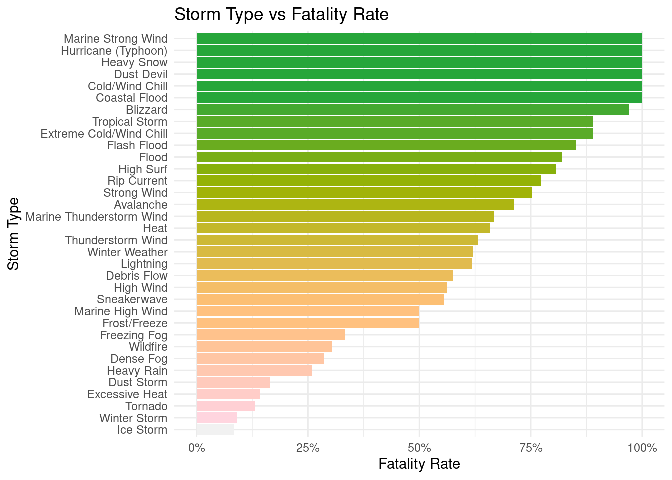
What storm types exhibit the highest fatality rates?
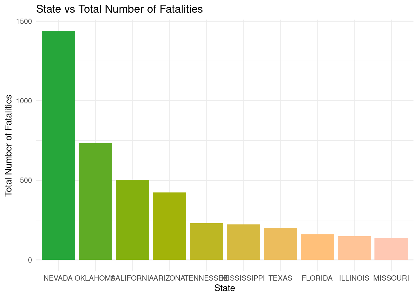
Which specific geographical locations experience the most fatalities as a result of storms?
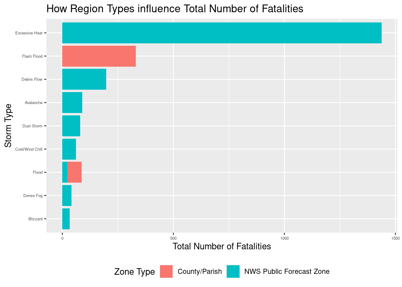
How do distinct storm types and varying geographical locations influence the number of fatalities?
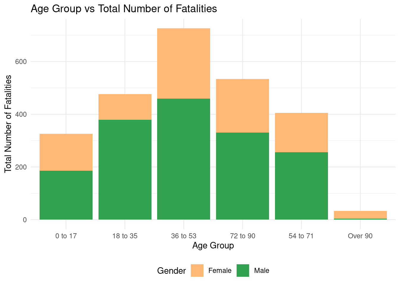
Is there a discernible pattern in the demographics of fatalities and damages based on storm types or locations?
How have the characteristics of storms, including their frequency, intensity, and locations, evolved throughout history? (Without adding fatalities, combine the 2003, 2013, 2023 data sets)
How have the begin time, end time, and duration time of storms influenced the number of fatalities?
How have the months of storms influenced the number of fatalities?
What are the potential strategies for minimizing storm-related fatalities and damages?
After all questions are answered
With this project, we will visualize storm characteristics and attribute correlations, uncovering patterns/trends through historical data; offer mitigation/awareness recommendations for future planning practices; and clearly present findings through data visualizations and reports.
Data collection and cleaning
Have an initial draft of your data cleaning appendix. Document every step that takes your raw data file(s) and turns it into the analysis-ready data set that you would submit with your final project. Include text narrative describing your data collection (downloading, scraping, surveys, etc) and any additional data curation/cleaning (merging data frames, filtering, transformations of variables, etc). Include code for data curation/cleaning, but not collection.
library(readr)library(tidyverse)
── Attaching core tidyverse packages ──────────────────────── tidyverse 2.0.0 ──
✔ dplyr     1.1.2     ✔ purrr     1.0.2
✔ forcats   1.0.0     ✔ stringr   1.5.0
✔ ggplot2   3.4.3     ✔ tibble    3.2.1
✔ lubridate 1.9.2     ✔ tidyr     1.3.0
── Conflicts ────────────────────────────────────────── tidyverse_conflicts() ──
✖ dplyr::filter() masks stats::filter()
✖ dplyr::lag()    masks stats::lag()
ℹ Use the conflicted package (<http://conflicted.r-lib.org/>) to force all conflicts to become errors
library(lubridate)library(scales)
Attaching package: 'scales'

The following object is masked from 'package:purrr':

    discard

The following object is masked from 'package:readr':

    col_factor
Rows: 52956 Columns: 51
── Column specification ────────────────────────────────────────────────────────
Delimiter: ","
chr (21): STATE, MONTH_NAME, EVENT_TYPE, CZ_TYPE, CZ_NAME, WFO, BEGIN_DATE_T...
dbl (24): BEGIN_YEARMONTH, BEGIN_DAY, BEGIN_TIME, END_YEARMONTH, END_DAY, EN...
lgl  (6): FLOOD_CAUSE, CATEGORY, TOR_OTHER_WFO, TOR_OTHER_CZ_STATE, TOR_OTHE...

ℹ Use `spec()` to retrieve the full column specification for this data.
ℹ Specify the column types or set `show_col_types = FALSE` to quiet this message.
all_2013 <-read_csv("data/2013.csv")
Warning: One or more parsing issues, call `problems()` on your data frame for details,
e.g.:
  dat <- vroom(...)
  problems(dat)
Rows: 59986 Columns: 51
── Column specification ────────────────────────────────────────────────────────
Delimiter: ","
chr (26): STATE, MONTH_NAME, EVENT_TYPE, CZ_TYPE, CZ_NAME, WFO, BEGIN_DATE_T...
dbl (24): BEGIN_YEARMONTH, BEGIN_DAY, BEGIN_TIME, END_YEARMONTH, END_DAY, EN...
lgl  (1): CATEGORY

ℹ Use `spec()` to retrieve the full column specification for this data.
ℹ Specify the column types or set `show_col_types = FALSE` to quiet this message.
all_2023 <-read_csv("data/2023.csv")
Rows: 38109 Columns: 51
── Column specification ────────────────────────────────────────────────────────
Delimiter: ","
chr (26): STATE, MONTH_NAME, EVENT_TYPE, CZ_TYPE, CZ_NAME, WFO, BEGIN_DATE_T...
dbl (24): BEGIN_YEARMONTH, BEGIN_DAY, BEGIN_TIME, END_YEARMONTH, END_DAY, EN...
lgl  (1): CATEGORY

ℹ Use `spec()` to retrieve the full column specification for this data.
ℹ Specify the column types or set `show_col_types = FALSE` to quiet this message.
f_2003 <-read_csv("data/2003f.csv")
Rows: 443 Columns: 11
── Column specification ────────────────────────────────────────────────────────
Delimiter: ","
chr (4): FATALITY_TYPE, FATALITY_DATE, FATALITY_SEX, FATALITY_LOCATION
dbl (7): FAT_YEARMONTH, FAT_DAY, FAT_TIME, FATALITY_ID, EVENT_ID, FATALITY_A...

ℹ Use `spec()` to retrieve the full column specification for this data.
ℹ Specify the column types or set `show_col_types = FALSE` to quiet this message.
f_2013 <-read_csv("data/2013f.csv")
Rows: 593 Columns: 11
── Column specification ────────────────────────────────────────────────────────
Delimiter: ","
chr (4): FATALITY_TYPE, FATALITY_DATE, FATALITY_SEX, FATALITY_LOCATION
dbl (7): FAT_YEARMONTH, FAT_DAY, FAT_TIME, FATALITY_ID, EVENT_ID, FATALITY_A...

ℹ Use `spec()` to retrieve the full column specification for this data.
ℹ Specify the column types or set `show_col_types = FALSE` to quiet this message.
f_2023 <-read_csv("data/2023f.csv")
Rows: 332 Columns: 11
── Column specification ────────────────────────────────────────────────────────
Delimiter: ","
chr (4): FATALITY_TYPE, FATALITY_DATE, FATALITY_SEX, FATALITY_LOCATION
dbl (7): FAT_YEARMONTH, FAT_DAY, FAT_TIME, FATALITY_ID, EVENT_ID, FATALITY_A...

ℹ Use `spec()` to retrieve the full column specification for this data.
ℹ Specify the column types or set `show_col_types = FALSE` to quiet this message.
all_strom <-rbind(all_2003, all_2013, all_2023)f_storm <-rbind(f_2003, f_2013, f_2023)f_storm <-left_join(f_storm, all_strom, by ="EVENT_ID") f_storm$BEGIN_DATE_TIME <-dmy_hms(f_storm$BEGIN_DATE_TIME)# Extract the time component from BEGIN_DATE_TIMEf_storm$time <-format(f_storm$BEGIN_DATE_TIME, format ="%H:%M:%S")# Convert the END_DATE_TIME variable to a date-time objectf_storm$END_DATE_TIME <-dmy_hms(f_storm$END_DATE_TIME)# Calculate the duration in secondsf_storm$Duration <-as.numeric(difftime(f_storm$END_DATE_TIME, f_storm$BEGIN_DATE_TIME, units ="secs"))f_storm_clean <-select(f_storm, "FATALITY_ID", "EVENT_ID", "FATALITY_TYPE", "FATALITY_AGE", "FATALITY_SEX", "FATALITY_LOCATION", "EPISODE_ID", "STATE", "YEAR", "MONTH_NAME", "EVENT_TYPE", "CZ_TYPE", "CZ_NAME", "BEGIN_DATE_TIME", "CZ_TIMEZONE", "END_DATE_TIME", "INJURIES_DIRECT", "INJURIES_INDIRECT", "DEATHS_DIRECT", "DEATHS_INDIRECT")
Data description
Storm Data, from the National Weather Service, offers comprehensive statistics on injuries and damage estimates for U.S. weather incidents from 1950 to the present. The NCDC Storm Event database categorizes various storms by type, state, and date. The NWS uses various data sources to enhance weather monitoring and forecasting. We selected representative years (2003, 2013, 2023) and merged 6 datasets, excluding prior years with missing entries and CSV errors in Storm Event Location data.
The full description of the storm data can be accessed in the PDF at this link: (https://www.ncei.noaa.gov/pub/data/swdi/stormevents/csvfiles/Storm-Data-Bulk-csv-Format.pdf).
The cleaned data includes 21 columns, each row represents a single fatality and includes personal details along with relevant storm events and episode information. This information is linked through the following ID numbers:
Fatality_ID, Event_ID, Episode_ID: These ID numbers are used to merge the datasets. An episode may contain multiple storm events and an episode is defined as the occurrence of storms and significant weather phenomena that can lead to loss of life, injuries, property damage, or disruption to commerce.
The time-related data includes:
Begin & end date time, CZ timezone: Specifies the start and end date and time of the storm event in the corresponding time zones.
Year, month: Indicates the year and month of the event.
The fatality-related data includes:
FATALITY_TYPE: Indicates whether the fatality is direct or indirect (D or I).
FATALITY_AGE: Numeric age of the person with the fatality.
FATALITY_SEX: Biological sex of the person with the fatality.
FATALITY_LOCATION: Specifies the location where the fatality occurred, including various categories such as Ball Field, Boating, Business, Camping, Church, Heavy Equipment/Construction, Golfing, In Water, Long Span Roof, Mobile/Trailer Home, Other/Unknown, Outside/Open Areas, Permanent Home, Permanent Structure, School, Telephone, Under Tree.
The event-related data includes:
STATE: The state in which the storm occurred.
Event type & CZ name & type: Describes the type of storm event that led to fatalities, injuries, damage, etc. It provides a detailed breakdown with corresponding designators, such as county or zone
Injuries direct & indirect, deaths direct & indirect: Records the number of direct and indirect injuries and deaths associated with the storm event.
The mixture of fatality and event-related variables in the dataset enables researchers to make correlations and draw inferences, especially when analyzing data over time, to answer specific questions related to storm events.
Data limitations
Our primary constraint is the limited amount of time and power available for dataset preparation. Given the extensive volume of information and the size of the original files, we are unable to incorporate additional timeframes into a single dataset. Consequently, our ability to draw historical inferences or unveil time-dependent patterns may be restricted. To address this, we have spread our data over a span of two decades, encompassing the years 2003, 2013, and 2023, ensuring the inclusion of data from substantial time periods.
Furthermore, the original dataset exhibits significant missing data for earlier years (before 2010s), with numerous columns containing missing information. Regrettably, some of these missing data would’ve been helpful for meaningful data analysis. Thus, we had to selectively retain only the most relevant columns, discarding many others with missing information. With the cleaned dataset, however, we’re confident that we can create valuable and insightful visualizations.
Exploratory data analysis
Q1: What storm types exhibit the highest fatality rates? (Label: Fatalities in Different Storms)
f_storm_clean_Q1 <- f_storm_clean |>select(EVENT_TYPE, INJURIES_DIRECT, INJURIES_INDIRECT, DEATHS_DIRECT, DEATHS_INDIRECT) |>mutate(sum = INJURIES_DIRECT + INJURIES_INDIRECT + DEATHS_DIRECT + DEATHS_INDIRECT,fatalities = DEATHS_DIRECT + DEATHS_INDIRECT ) |>group_by(EVENT_TYPE) |>summarize(total =sum(sum),total_fatalities =sum(fatalities),rate = total_fatalities / total ) |>drop_na() |>arrange(desc(rate))f_storm_clean_Q1 |>ggplot(mapping =aes(x =reorder(EVENT_TYPE, rate), y = rate, fill =factor(-rate))) +geom_col(show.legend =FALSE) +scale_fill_manual(values =paletteer_c("grDevices::Terrain", 27)) +labs(x ='Storm Type', y ='Fatality Rate', title ='Storm Type vs Fatality Rate') +scale_y_continuous(labels =label_percent(suffix ='%')) +theme_minimal()+coord_flip()
Q2: Which specific geographic location (state) experiences the most fatalities as a result of storms?
f_storm_clean_Q2 <- f_storm_clean |>select(STATE, DEATHS_DIRECT, DEATHS_INDIRECT) |>mutate(fatalities = DEATHS_DIRECT + DEATHS_INDIRECT ) |>group_by(STATE) |>summarize(sum =sum(fatalities) ) |>arrange(desc(sum)) |>head(10)f_storm_clean_Q2 |>ggplot(mapping =aes(x =reorder(STATE, -sum), y = sum, fill =factor(-sum))) +geom_col(show.legend =FALSE) +scale_fill_manual(values =paletteer_c("grDevices::Terrain", 12)) +labs(x ='State', y ='Total Number of Fatalities', title ='State vs Total Number of Fatalities') +theme(axis.text =element_text(size =4)) +theme_minimal()
Q3: How do distinct storm types and varying geological locations influence the number of fatalities?
`summarise()` has grouped output by 'EVENT_TYPE'. You can override using the
`.groups` argument.
f_storm_clean_Q3 |>ggplot(mapping =aes(x =reorder(EVENT_TYPE, sum), y = sum, fill = CZ_TYPE)) +geom_bar(stat ="identity") +labs(x ='Storm Type', y ='Total Number of Fatalities', title ='How Region Types influence Total Number of Fatalities',fill ='Zone Type') +theme(axis.text =element_text(size =5)) +theme(legend.position ='bottom') +scale_fill_discrete(labels =c('County/Parish', 'NWS Public Forecast Zone')) +coord_flip()
Q4: Is there a discernible pattern in the demographics (age) of fatalities and damages based on storm types or locations?
`summarise()` has grouped output by 'FATALITY_SEX'. You can override using the
`.groups` argument.
f_storm_clean_Q4 |>ggplot(mapping =aes(x = age_group, y = sum, fill =factor(FATALITY_SEX))) +geom_col() +scale_fill_manual(values =c("#FFB977", "#32A251"),labels =c('Female', 'Male')) +scale_x_discrete(labels =c('0 to 17', '18 to 35', '36 to 53','72 to 90','54 to 71','Over 90')) +theme_minimal()+theme(legend.position ='bottom') +labs(x ='Age Group', y ='Total Number of Fatalities', title ='Age Group vs Total Number of Fatalities',fill ='Gender')
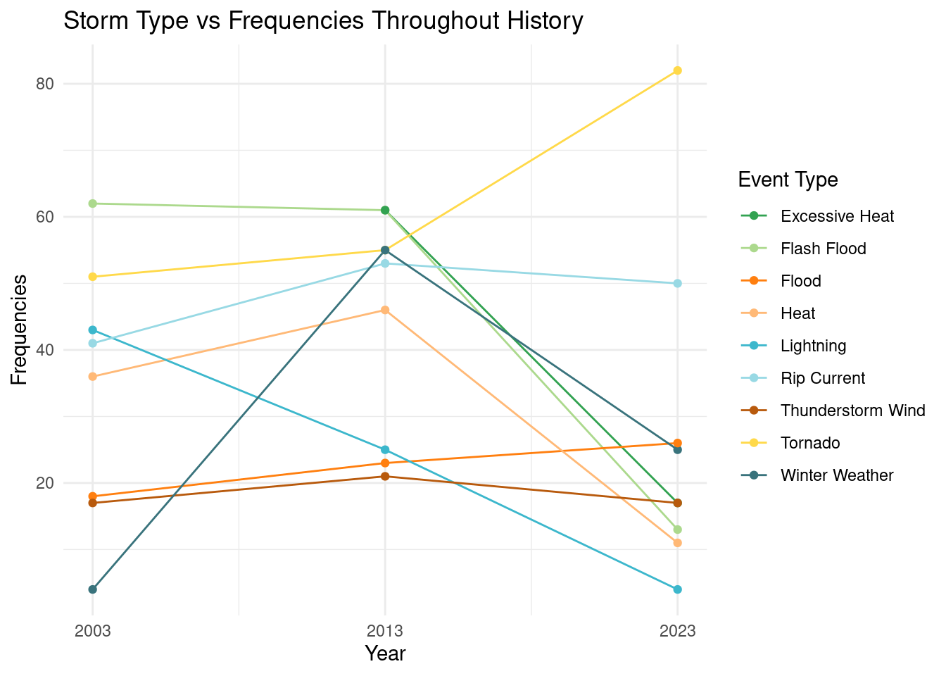
Q5: How have the characteristics of storms and their frequency evolved throughout history?
`summarise()` has grouped output by 'EVENT_TYPE'. You can override using the
`.groups` argument.
# Frequenciesf_storm_clean_Q5 |>ggplot(mapping =aes(x = YEAR, y = FREQUENCY, color = EVENT_TYPE)) +geom_line() +geom_point() +scale_color_manual(values =paletteer_d("ggthemes::Classic_Green_Orange_12")) +labs(x ='Year', y ='Frequencies', title ='Storm Type vs Frequencies Throughout History',fill ='Year', color ='Event Type') +theme(text =element_text(size =6)) +scale_x_continuous(breaks =seq(2003, 2023, by =10)) +theme_minimal()
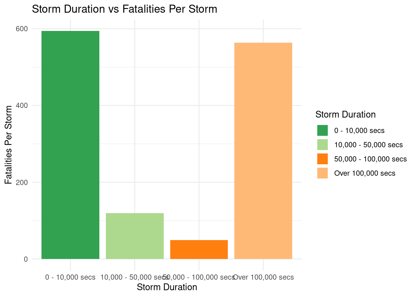
Q6: How have the begin time, end time, and duration time of storms influenced the number of fatalities?
Warning: Using `size` aesthetic for lines was deprecated in ggplot2 3.4.0.
ℹ Please use `linewidth` instead.
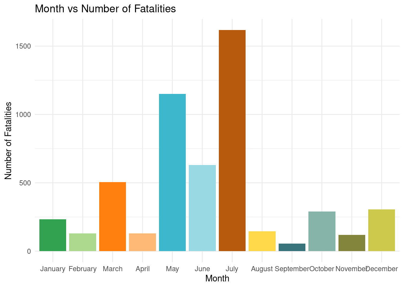
Q7: How have the months of storms influenced the number of fatalities?
f_storm_clean_Q7 <- f_storm_clean |>select(MONTH_NAME, DEATHS_DIRECT, DEATHS_INDIRECT) |>mutate(fatalities = DEATHS_DIRECT + DEATHS_INDIRECT,MONTH_NAME =factor(MONTH_NAME, levels = month.name) ) |>drop_na() |>group_by(MONTH_NAME) |>summarise(total =sum(fatalities) )f_storm_clean_Q7 |>ggplot(mapping =aes(x = MONTH_NAME, y = total, fill = MONTH_NAME)) +geom_col(size =25, show.legend =FALSE) +scale_fill_manual(values =paletteer_d("ggthemes::Classic_Green_Orange_12")) +theme(legend.position ='none') +labs(x ='Month', y ='Number of Fatalities',title ='Month vs Number of Fatalities') +theme(text =element_text(size =8)) +theme_minimal()
Shiny App Updates
For this part, we will briefly describe what we will do with the help of ShinyApp. We will develop a dashboard that can show both data information and plots. For “Ui” section, it is responsible for showing the data, and for “Server” section, it is responsible for processing data.
By clicking different buttons or even menu information on the sidebar, we can see information we want, and exclude the information we don’t need at this time.
For our project, we can build a part that can reflect the data change in real-time, which maybe on the very top of the screen. Moreover, we can create different plots by clicking different storm evens we want, and show detailed information like how many people get injured and the fatalities information and so on. We can also generate comparison information and show time-series information about that.
Apart from that, we will leave space for word descriptions, to make our presentation more complete and more understandable.
Questions for reviewers
Does the selection of representative years (2003, 2013, 2023) provide a sufficient time span for analyzing historical trends in storm behavior? Are there any concerns or suggestions regarding the choice of these years?
Are there any ethical considerations or privacy concerns that should be taken into account when working with personal details and fatality-related data? How can these concerns be addressed and ensured in the project?