#|label: load-package-data
#|cache: false


# Load the readr package
library(readr)
library(tidyverse)
library(scales)
library(janitor)
library(lubridate)
library(reshape2)

# Read the CSV file
djcigc <- read_csv(here::here("data/DJCIGC.csv"), show_col_types = FALSE)
dxy <- suppressWarnings(read_csv(here::here(file = "data/DXY.csv"),
  show_col_types = FALSE
))
ixic <- suppressWarnings(read_csv(here::here(file = "data/IXIC.csv"),
  show_col_types = FALSE
))
gspc <- suppressWarnings(read_csv(here::here(file = "data/ GSPC.csv"),
  show_col_types = FALSE
))
bnb <- suppressWarnings(read_csv(
  here::here(
    file =
      "data/Binance_BNBUSDT_d.csv"
  ),
  skip = 1, show_col_types = FALSE
))
btc <- suppressWarnings(read_csv(
  here::here(
    file =
      "data/Binance_BTCUSDT_d.csv"
  ),
  skip = 1, show_col_types = FALSE
))
doge <- suppressWarnings(read_csv(
  here::here(
    file =
      "data/Binance_DOGEUSDT_d.csv"
  ),
  skip = 1, show_col_types = FALSE
))
eth <- suppressWarnings(read_csv(
  here::here(
    file =
      "data/Binance_ETHUSDT_d.csv"
  ),
  skip = 1, show_col_types = FALSE
))
uni <- suppressWarnings(read_csv(
  here::here(
    file =
      "data/Binance_UNIUSDT_d.csv"
  ),
  skip = 1, show_col_types = FALSE
))Cryptocurrency Digger
Exploration
Objective(s)
The objectives of this project:
Demonstrate the correlation, if any, between the major cryptocurrencies and the real-world key macroeconomic indicators.
Construct a machine learning model to do feature selection, and attempt to predict the behavior of the cryptocurrency based on selected features(real world economic indicators)
Employ an interactive tool(shiny) to allow researchers to interactively select real world economic indicators and cryptocurrencies on an interactive plot. They will be able to adjust timelines, drag and drop different dimensions, etc.
Data collection and cleaning
We have four team members and we divided our team into two sub-groups. Shiyi and Yushan were responsible for searching economic indicators, such as, S&P 500, NASDAQ composite index and US Dollar index, etc., which might have a meaningful impact on the price of crypto currency. Yichen and Qingyao aimed to find the price, price range and trading volume of the top 5 cryptocurrency.
The inflation rate monthly data was exported from https://www.usinflationcalculator.com/inflation/historical-inflation-rates/ . In order to match the time sequence of cryptocurrency, we assume that the inflation rate remains the same for each month in daily.
As for other indices like S&P 500, we found the data in https://finance.yahoo.com/ and https://fred.stlouisfed.org/ , the raw data contains open, close, highest and lowest etc. After discussion, we decided to focus on close price.
We found the data for crypto currency in https://www.cryptodatadownload.com. The data for a particular crypto currency is in daily format, and it contains price, volume, and fluctuation information.
When tidying the data, we initially utilized the mutate() function to extract the columns we needed, particularly the date column, from the raw datasets. We cleaned these columns individually within a single pipe. For instance, we encountered date data in various structures, some as numbers, others as characters. To facilitate the final joining process, we converted them all to the same data structure “date”. Additionally, we also create a date dataframe from 01/03/2017 to 09/29/2023 to standardize each raw data set.
#|label: combine data
#|cache: false
#|message: false
#|warning: false

# Extract date and price
# from Dow Jones Commodity Gold Historical Data dataframe
# Clean Dow Jones Commodity Gold Historical Data data frame
djcigc <- djcigc |>
  clean_names() |>
  select(date, price) |>
  mutate(
    date = as.Date(date, format = "%m/%d/%Y")
  ) |>
  arrange(date) |>
  rename(djcigc_price = "price")

# Extract date and close price from US Dollar Index dateframe
# Clean US Dollar Index dateframe

dxy <- dxy |>
  clean_names() |>
  select(date, close) |>
  mutate(
    close = suppressWarnings(coalesce(as.numeric(close), 0))
  ) |>
  rename(dxy_price = "close")

# Clean S&P500 dateframe
gspc <- gspc |>
  clean_names() |>
  mutate(
    sp500 = suppressWarnings(replace(as.numeric(sp500), sp500 == ".", 0))
  )
# Extract date and close price from NASDAQ COMPOSITE dataframe
# Clean NASDAQ COMPOSITE dataframe
ixic <- ixic |>
  clean_names() |>
  select(date, close) |>
  rename(ixic_price = "close")

btc <- btc |>
  clean_names() |>
  mutate(
    btc_flux = abs(high - low),
    date = as.Date(date, format = "%m/%d/%Y")
  ) |>
  select(date, close, volume_usdt, btc_flux) |>
  rename(btc_price = "close", btc_volume_usdt = "volume_usdt")

bnb <- bnb |>
  clean_names() |>
  mutate(
    bnb_flux = abs(high - low),
    date = as.Date(date, format = "%m/%d/%Y")
  ) |>
  select(date, close, volume_usdt, bnb_flux) |>
  rename(bnb_price = "close", bnb_volume_usdt = "volume_usdt")


doge <- doge |>
  clean_names() |>
  mutate(
    doge_flux = abs(high - low),
    date = as.Date(date, format = "%m/%d/%Y")
  ) |>
  select(date, close, volume_usdt, doge_flux) |>
  rename(doge_price = "close", doge_volume_usdt = "volume_usdt")

eth <- eth |>
  clean_names() |>
  mutate(
    eth_flux = abs(high - low),
    date = as.Date(date, format = "%m/%d/%Y")
  ) |>
  select(date, close, volume_usdt, eth_flux) |>
  rename(eth_price = "close", eth_volume_usdt = "volume_usdt")

uni <- uni |>
  clean_names() |>
  mutate(
    uni_flux = abs(high - low),
    date = as.Date(date, format = "%m/%d/%Y")
  ) |>
  select(date, close, volume_usdt, uni_flux) |>
  rename(uni_price = "close", uni_volume_usdt = "volume_usdt")


# change monthly data to daily data
monthly <- data.frame(
  Year = rep(2017:2023, each = 12), # Years 2017 to 2023
  Month = rep(1:12, times = 7), # Months from 1 to 12
  Monthly_Rate = c(
    2.5, 2.7, 2.4, 2.2, 1.9, 1.6, 1.7, 1.9, 2.2, 2, 2.2, 2.1,
    2.1, 2.2, 2.4, 2.5, 2.8, 2.9, 2.9, 2.7, 2.3, 2.5, 2.2, 1.9,
    1.6, 1.5, 1.9, 2, 1.8, 1.6, 1.8, 1.7, 1.7, 1.8, 2.1, 2.3,
    2.5, 2.3, 1.5, 0.3, 0.1, 0.6, 1, 1.3, 1.4, 1.2, 1.2, 1.4,
    1.4, 1.7, 2.6, 4.2, 5, 5.4, 5.4, 5.3, 5.4, 6.2, 6.8, 7,
    7.5, 7.9, 8.5, 8.3, 8.6, 9.1, 8.5, 8.3, 8.2, 7.7, 7.1, 6.5,
    6.4, 6, 5, 4.9, 4, 3, 3.2, 3.7, 3.7, 0, 0, 0
  )
)

# Create an empty data frame for daily data
inflation_data <- data.frame(
  date = as.Date(character(0)),
  inflation_rate = numeric(0)
)

# Loop through each row in monthly
for (i in 1:nrow(monthly)) {
  # Get the current year, month, and rate
  current_year <- monthly$Year[i]
  current_month <- monthly$Month[i]
  current_rate <- monthly$Monthly_Rate[i]

  # Calculate the last day of the current month
  last_day <- ceiling_date(
    ymd(paste(current_year, current_month, 1)),
    "month"
  ) - days(1)

  # Create daily data for the current month
  days_in_month <- seq(
    as.Date(paste(current_year,
      current_month, 1,
      sep = "-"
    )),
    to = last_day, by = "days"
  )

  monthly_data <- data.frame(
    date = days_in_month, inflation_rate =
      rep(current_rate, length(days_in_month))
  )

  # Append the monthly data to the daily_data data frame
  inflation_data <- rbind(inflation_data, monthly_data)
}

# Define the start and end dates for your desired date range
start_date <- as.Date("2017-01-03")
end_date <- as.Date("2023-09-29")

# Create a data frame with the complete date sequence
complete_dates <- data.frame(date = seq.Date(start_date, end_date,
  by = "days"
))

# Merge the complete date
# Sequence with  Dow Jones Commodity Gold Historical Data
djcigc <- complete_dates |>
  left_join(djcigc, by = "date")

djcigc[is.na(djcigc$djcigc_price), "djcigc_price"] <- 0

# Merge the complete date sequence with US Dollar Index dateframe
dxy <- complete_dates |>
  left_join(dxy, by = "date")

dxy[is.na(dxy$dxy_price), "dxy_price"] <- 0

# Merge the complete date sequence with S&P500 dateframe
gspc <- complete_dates |>
  left_join(gspc, by = "date")

gspc[is.na(gspc$sp500), "sp500"] <- 0

# Merge the complete date sequence with NASDAQ COMPOSITE dataframe
ixic <- complete_dates |>
  left_join(ixic, by = "date")

ixic[is.na(ixic$ixic_price), "ixic_price"] <- 0

# Merge the complete date sequence with inflation rate dataframe
inflation_data <- complete_dates |>
  left_join(inflation_data, by = "date")

inflation_data[
  is.na(inflation_data$inflation_rate),
  "inflation_rate"
] <- 0

btc <- complete_dates |>
  left_join(btc, by = "date") |>
  mutate(
    btc_price = if_else(is.na(btc_price), 0, btc_price),
    btc_volume_usdt = if_else(is.na(btc_volume_usdt), 0,
      btc_volume_usdt
    ),
    btc_flux = if_else(is.na(btc_flux), 0, btc_flux)
  )

eth <- complete_dates |>
  left_join(eth, by = "date") |>
  mutate(
    eth_price = if_else(is.na(eth_price), 0, eth_price),
    eth_volume_usdt = if_else(is.na(eth_volume_usdt), 0, eth_volume_usdt),
    eth_flux = if_else(is.na(eth_flux), 0, eth_flux)
  )
uni <- complete_dates |>
  left_join(uni, by = "date") |>
  mutate(
    uni_price = if_else(is.na(uni_price), 0, uni_price),
    uni_volume_usdt = if_else(is.na(uni_volume_usdt), 0, uni_volume_usdt),
    uni_flux = if_else(is.na(uni_flux), 0, uni_flux)
  )
doge <- complete_dates |>
  left_join(doge, by = "date") |>
  mutate(
    doge_price = if_else(is.na(doge_price), 0, doge_price),
    doge_volume_usdt = if_else(is.na(doge_volume_usdt), 0, doge_volume_usdt),
    doge_flux = if_else(is.na(doge_flux), 0, doge_flux)
  )
bnb <- complete_dates |>
  left_join(bnb, by = "date") |>
  mutate(
    bnb_price = if_else(is.na(bnb_price), 0, bnb_price),
    bnb_volume_usdt = if_else(is.na(bnb_volume_usdt), 0, bnb_volume_usdt),
    bnb_flux = if_else(is.na(bnb_flux), 0, bnb_flux)
  )
# Join mutilple dataframe
indices <- djcigc |>
  inner_join(dxy, by = "date") |>
  inner_join(gspc, by = "date") |>
  inner_join(ixic, by = "date") |>
  inner_join(inflation_data, by = "date") |>
  inner_join(btc, by = "date") |>
  inner_join(bnb, by = "date") |>
  inner_join(eth, by = "date") |>
  inner_join(uni, by = "date") |>
  inner_join(doge, by = "date")
Data description
Our cleaned dataset, called ‘exploration_data_cleaned,’ consists of 2,461 rows and 21 columns.
date [date]:the date between 01/03/2017 and 09/29/2023
djcigc_price [double]: close price from Dow Jones Commodity Gold Historical Data
dxy_price [double]: close price from US Dollar Index Historical Data
sp500 [double]: the price is calculated based on the market cap of ~500 publicly traded U.S. companies, which is equal to the share price of the company multiplied by the total number of shares outstanding.
Ixic_price [double]: close price from NASDAQ COMPOSITE Historical Data
inflation_rate [double]: U.S. inflation rate
btc_price [double]: historical close price of Bitcoin
btc_volume_usdt [double]: daily trading volume of Bitcoin (based on US dollar)
btc_flux [double]: daily price range of Bitcoin
bnb_price [double]: historical close price of Binance Coin
bnb_volume_usdt [double]: daily trading volume of Binance Coin (based on US dollar)
bnb_flux [double]: daily price range of Binance Coin
eth_price [double]: historical close price of Ethereum
eth_volume_usdt [double]: daily trading volume of Ethereum (based on US dollar)
eth_flux [double]: daily price range of Ethereum
uni_price [double]: historical close price of Uniswap Token
uni_volume_usdt [double]: daily trading volume of Uniswap Token (based on US dollar)
uni_flux [double]: daily price range of Uniswap Token
doge_price [double]: historical close price of Dogecoin
doge_volume_usdt [double]: daily trading volume of Dogecoin (based on US dollar)
doge_flux [double]: daily price range of Dogecoin
Data limitations
- Time frame Mismatch:
Bitcoin data and economic indicators may have different timeframes or frequencies. For example, Bitcoin price data may be available on a daily basis, while economic indicators are reported monthly or quarterly. You’ll need to address this discrepancy to ensure meaningful analysis.
- Currency and Exchange Rate Issues:
Bitcoin prices are typically quoted in various fiat currencies, and exchange rate fluctuations can affect the value of Bitcoin. If you’re using economic indicators from different countries, exchange rate changes can introduce noise into your analysis.
- Unavailable data:
Some of the crypto currencies did not emerge until 2020, our time frame of interest starts in 2017. So we would have to put 0 to replace NA. This could be problematic if we want to conclude something more general for all crypto currencies.
Exploratory data analysis
Perform an (initial) exploratory data analysis.
#|label: Exploratory Data Analysis and Data Normalization

# Specify the path to the CSV file
data_file_path <- here::here("data/exploration_data_cleaned.csv")

# Read the 'exploration_data_cleaned' dataset from the CSV file
exploration_data_cleaned <- read_csv(data_file_path)

#load necessary libraries
library(ggplot2)
library(recipes)

# Create a recipe for normalization
normalization_recipe <- exploration_data_cleaned |>
  select(-date)|>
  recipe(~ .) |>
  step_normalize(all_predictors())

# Prepare the recipe (estimate parameters)
prepped_recipe <- prep(normalization_recipe)

# Apply the prepped recipe to the entire dataset
normalized_data <- bake(prepped_recipe, new_data = exploration_data_cleaned)
joined_data <- cbind(exploration_data_cleaned$date, normalized_data)
colnames(joined_data)[1] <- "date"

# Create a ggplot object
ggplot(joined_data, aes(x = date)) +

  # Add points for dxy_price
  geom_line(aes(y = dxy_price, color = "Binance Coin")) +

  # Add points for btc_price
  geom_line(aes(y = btc_price, color = "Btc Price")) +

  # Customize the plot (optional)
  labs(title = "ETC, BNB, and BTC Prices Over Time",
       x = "Date",
       y = "Price",
       color = "Cryptocurrency") +

  theme_minimal()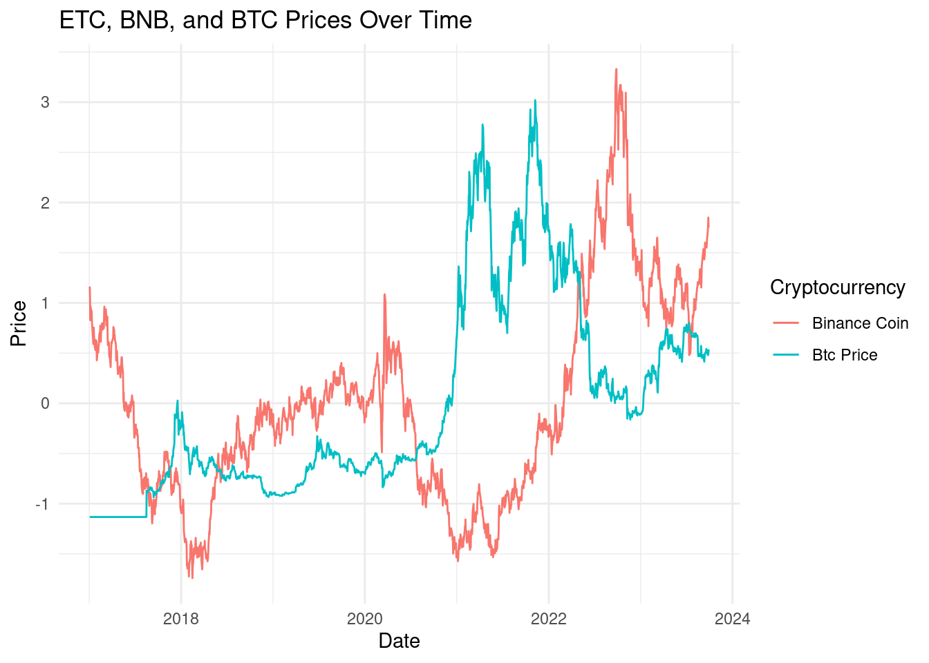
#exports the joined_data data frame to a CSV file, excluding row names, and saves it in the "data" directory with the filename "joined_data.csv"
write.csv(joined_data, "data/joined_data.csv", row.names = FALSE)
During our initial exploratory analysis, we compared the price trend of Bitcoin (btc_price) with four other economic indices of interest: djcigc_price, dxy_price, Sp500, and Ixic_price, on a monthly basis throughout the year 2020. The graphical analysis revealed that all five variables exhibit similar trends, with notable patterns emerging.
Specifically, the price trends of gold (gold price) and the U.S. Dollar Index (dxy_price) closely paralleled each other, while the S&P 500 (Sp500) and the NASDAQ Composite (Ixic_price) demonstrated comparable trends. In contrast, Bitcoin’s price trend stood out during three specific months: May (2020-05), August (2020-08), and November (2020-11). In these months, Bitcoin’s price increased while the prices of the other four indices declined. This observation is of significance and warrants further analysis to comprehend why Bitcoin exhibited distinct trends during these particular months, while other indices displayed opposing trends. This aspect will be explored in greater detail in subsequent research.
The choice of the year 2020 for our exploration is attributed to the global crises and uncertainties that characterized this period, primarily due to the COVID-19 pandemic. These uncertainties potentially led investors to seek refuge in safe-haven assets, with Bitcoin being likened to digital gold, consequently garnering heightened interest.
In the realm of macroeconomic factors, 2020 witnessed global economic turbulence on an unprecedented scale. Central banks implemented expansive stimulus measures, substantially easing monetary policies, which may have exerted an influence on Bitcoin’s price. Bitcoin is acknowledged as a non-traditional safe-haven asset capable of hedging against inflation.
#|label: Data preparation/preprocessing for machine learning

# Read Bitcoin (BTC) data from CSV and perform initial cleaning
btc_ml <- suppressWarnings(read_csv(
  here::here(
    file =
      "data/Binance_BTCUSDT_d.csv"
  ),
  skip = 1, show_col_types = FALSE
))

# Data manipulation for Bitcoin (BTC)
btc_ml <- btc_ml |>
  clean_names() |>
  mutate(
    btc_trend = if_else((close-open)>=0,TRUE,FALSE),
    date = as.Date(date, format = "%m/%d/%Y")
  ) |>
  select(date, close, volume_usdt, btc_trend) |>
  rename(btc_price = "close", btc_volume_usdt = "volume_usdt")

# Complete missing dates and join with Bitcoin (BTC) data
btc_ml <- complete_dates |>
  left_join(btc_ml, by = "date") |>
  mutate(
    btc_price = if_else(is.na(btc_price), 0, btc_price),
    btc_volume_usdt = if_else(is.na(btc_volume_usdt), 0,
      btc_volume_usdt
    )
  )

# Read Gold data and perform data manipulation
Gold_ML <- read_csv("data/DJCIGC.csv", col_types = cols(`Change %` = col_number()))
Gold_ML <- Gold_ML |>
  clean_names() |>
  mutate(
    gold_trend = if_else(change_percent>=0,TRUE,FALSE),
    date = as.Date(date, format = "%m/%d/%Y")
  ) |>
  select(date, open, gold_trend) |>
  rename(gold_price = "open")

# Complete missing dates and join with Gold data
Gold_ML <- complete_dates |>
  left_join(Gold_ML, by = "date")

# Read Dollar Index (DXY) data and perform data manipulation
Dollar_ML <- read_csv("data/DXY.csv",
                       na = "null",
                       col_types = cols(`open` = col_number(),
                                        `close` = col_number()))
Warning: The following named parsers don't match the column names: open, closeDollar_ML <- Dollar_ML |>
clean_names() |>
mutate(
dollar_trend = if_else(close - open >= 0,TRUE,FALSE),
date = as.Date(date, format = "%m/%d/%Y")
) |>
select(date,open, close, dollar_trend)
# Prepare Inflation data
Inflation_ML <- exploration_data_cleaned |>
select(date,inflation_rate) |>
mutate(
inflation_level = if_else(inflation_rate >= 2,TRUE,FALSE),
date = as.Date(date, format = "%m/%d/%Y")
) |>
select(date, inflation_rate, inflation_level)
# Merge all datasets into ml_prep for machine learning
ml_prep <- djcigc |>
inner_join(dxy, by = "date") |>
inner_join(ixic, by = "date") |>
inner_join(btc_ml, by = "date")|>
inner_join(Inflation_ML, by ="date")|>
drop_na()
# Load xgboost library
library(xgboost)
Attaching package: 'xgboost'The following object is masked from 'package:dplyr':
slice# Read imputed Gold data for testing and perform data manipulation
imputed_gold_test <- read_csv("data/imputed_Gold_ML.csv")Rows: 2461 Columns: 3── Column specification ────────────────────────────────────────────────────────
Delimiter: ","
dbl (1): gold_price
lgl (1): gold_trend
date (1): date
ℹ Use `spec()` to retrieve the full column specification for this data.
ℹ Specify the column types or set `show_col_types = FALSE` to quiet this message.ml_prep_test <- imputed_gold_test |>
inner_join(btc_ml, by = "date") |>
inner_join(Dollar_ML, by = "date") |>
inner_join(Inflation_ML, by ="date")|>
drop_na()#|label: Build XGBoost Classification Workflow
# Load necessary libraries
library(parsnip)
library(tidymodels)── Attaching packages ────────────────────────────────────── tidymodels 1.1.0 ──✔ broom 1.0.5 ✔ tune 1.1.1
✔ dials 1.2.0 ✔ workflows 1.1.3
✔ infer 1.0.4 ✔ workflowsets 1.0.1
✔ modeldata 1.2.0 ✔ yardstick 1.2.0
✔ rsample 1.1.1 ── Conflicts ───────────────────────────────────────── tidymodels_conflicts() ──
✖ scales::discard() masks purrr::discard()
✖ dplyr::filter() masks stats::filter()
✖ recipes::fixed() masks stringr::fixed()
✖ dplyr::lag() masks stats::lag()
✖ xgboost::slice() masks dplyr::slice()
✖ yardstick::spec() masks readr::spec()
✖ recipes::step() masks stats::step()
• Dig deeper into tidy modeling with R at https://www.tmwr.orglibrary(themis)
# Convert categorical variables to factors
ml_prep_test<- ml_prep_test |>
mutate(
btc_trend = factor(btc_trend),
gold_trend = factor(gold_trend),
dollar_trend = factor(dollar_trend),
inflation_level = factor(inflation_level)
)
# Split the data into training and testing sets
test_split <- initial_split(data = ml_prep_test, prop = 4/5)
test_train <- training(test_split)
test_test <- testing(test_split)
# Add a new row to the testing set and save it as an RDS file
test_test <- test_test |>
rbind(list(today(), 2063.6, FALSE, 41465.5, 33866922434, TRUE, 103.18, 103.73, TRUE, 3.24, TRUE)) |>
filter(btc_volume_usdt == 33866922434)
#saveRDS(test_test, "testdata.rds")
# Set up XGBoost model and k-Nearest Neighbors model
xgb_test <- boost_tree(engine = "xgboost") |>
set_mode("classification")
# Create cross-validation folds for model evaluation
test_folds <- vfold_cv(data = test_train, v = 10)
# Prepare the recipe for XGBoost
xgb_rec <- recipe(btc_trend ~ ., data = test_train) |>
step_rm(date, gold_price, gold_trend,) |>
step_dummy(all_nominal_predictors()) |>
step_zv(all_predictors()) |>
step_normalize(all_numeric()) |>
step_downsample(btc_trend)
# Set up the workflow with the recipe and model
xgb_wf <- workflow() |>
add_recipe(xgb_rec) |>
add_model(xgb_test)
# Set seed for reproducibility
set.seed(100)
# Fit the model using resampling (cross-validation)
modelout <- xgb_wf |>
fit_resamples(resamples = test_folds,
metrics = metric_set(roc_auc),
control = control_resamples(save_workflow = TRUE))
# Get the best model from resampling
mdbest <- fit_best(modelout)
# Make predictions on the new data
predstoday<- bind_cols(
test_test,
predict(mdbest, new_data = test_test, type = "class")
)
# Write the predictions to a CSV file
#write.csv(predstoday, "data/today_data.csv", row.names = FALSE)#|label: Save Best Model as RDS
# Save the best model obtained from resampling as an RDS file
#saveRDS(mdbest, "saved_model.rds")Questions for reviewers
- What will be a good machine learning model that best serves our purposes?
- How will you wish to interact with our shiny deliverable?
- What do you think is a good time to buy bitcoin?