library(tidyverse)
library(skimr)
library(readr)Earthquakes Around the World
Exploration
Objective(s)
We want to explore the relationship between time, location, and magnitude of earthquakes in the past year around the globe.
Data collection and cleaning
Step 1: Read Data
earthquakes_1 <- read_csv("./data/earthquakes_1.csv")Rows: 13389 Columns: 22
── Column specification ────────────────────────────────────────────────────────
Delimiter: ","
chr (8): magType, net, id, place, type, status, locationSource, magSource
dbl (12): latitude, longitude, depth, mag, nst, gap, dmin, rms, horizontalE...
dttm (2): time, updated
ℹ Use `spec()` to retrieve the full column specification for this data.
ℹ Specify the column types or set `show_col_types = FALSE` to quiet this message.earthquakes_2 <- read_csv("./data/earthquakes_2.csv")Rows: 13545 Columns: 22
── Column specification ────────────────────────────────────────────────────────
Delimiter: ","
chr (8): magType, net, id, place, type, status, locationSource, magSource
dbl (12): latitude, longitude, depth, mag, nst, gap, dmin, rms, horizontalE...
dttm (2): time, updated
ℹ Use `spec()` to retrieve the full column specification for this data.
ℹ Specify the column types or set `show_col_types = FALSE` to quiet this message.Step 2: Combine 2 dataframes
earthquakes <- rbind(earthquakes_1, earthquakes_2)
glimpse(earthquakes)
Rows: 26,934
Columns: 22
$ time <dttm> 2022-06-30 23:59:30, 2022-06-30 23:46:30, 2022-06-30 …
$ latitude <dbl> 19.48600, 7.30270, 64.51070, 4.95280, -2.68440, 38.899…
$ longitude <dbl> -66.34467, -79.98290, -138.43050, -76.08950, 109.98740…
$ depth <dbl> 8.490, 10.000, 11.200, 114.035, 10.000, 35.000, 124.51…
$ mag <dbl> 3.35, 4.40, 3.10, 4.50, 4.30, 4.10, 3.60, 4.20, 4.60, …
$ magType <chr> "md", "mb", "ml", "mb", "mb", "mb", "mb", "mb", "mb", …
$ nst <dbl> 15, 52, NA, 82, 29, 26, 24, 19, 63, 31, 22, 19, 15, 16…
$ gap <dbl> 254.00, 128.00, NA, 93.00, 120.00, 132.00, 110.00, 131…
$ dmin <dbl> NA, 3.0610, NA, 1.3510, 4.3600, 2.1820, 0.1850, 2.2080…
$ rms <dbl> 0.4100, 0.8300, 0.7100, 0.6200, 0.5800, 0.8800, 0.3500…
$ net <chr> "pr", "us", "ak", "us", "us", "us", "us", "us", "us", …
$ id <chr> "pr71356838", "us6000hyzk", "ak0228bq8in8", "us6000hyz…
$ updated <dttm> 2022-07-01 00:31:37, 2022-09-03 21:03:23, 2022-08-21 …
$ place <chr> "112 km N of Brenas, Puerto Rico", "25 km S of Pedasí,…
$ type <chr> "earthquake", "earthquake", "earthquake", "earthquake"…
$ horizontalError <dbl> 2.75, 5.57, NA, 4.40, 9.62, 7.41, 5.00, 4.70, 9.30, 7.…
$ depthError <dbl> 4.300, 1.755, 0.700, 6.290, 1.886, 1.922, 3.800, 8.900…
$ magError <dbl> 0.16929281, 0.08000000, NA, 0.04500000, 0.13300000, 0.…
$ magNst <dbl> 11, 45, NA, 143, 16, 10, 4, 9, 55, 12, 14, 4, 14, 15, …
$ status <chr> "reviewed", "reviewed", "reviewed", "reviewed", "revie…
$ locationSource <chr> "pr", "us", "ak", "us", "us", "us", "us", "us", "us", …
$ magSource <chr> "pr", "us", "ak", "us", "us", "us", "us", "us", "us", …Step 3: Remove Unnecessary Columns and rename others
earthquakes <- earthquakes |>
  select(!c(magType, nst, rms, id, updated, horizontalError, depthError, magError, magNst,  locationSource, magSource)) |>
  rename(
    "magnitude" = "mag",
    "min_dis_to_center" = "dmin",
    "source" = "net"
  ) |>
  filter(
    !is.na(longitude) & !is.na(latitude)
  )
Step 4: Extract date information
earthquakes <- earthquakes |>
  mutate(
    time = ymd_hms(time),
    year = year(time),
    month = month(time, label = TRUE),
    day = day(time),
    .after = time
    ) |>
  mutate(
    month = match(month, month.abb)
  )
Step 5: Convert to numeric/char and create a separate country column
earthquakes <- earthquakes |>
  mutate(
    across(latitude:min_dis_to_center, as.numeric)
  )
us_states = list("Alabama", "Alaska", "Arizona", "Arkansas", "California", "Colorado", "Connecticut", "Delaware", "Florida", "Georgia", "Hawaii", "Idaho", "Illinois", "Indiana", "Iowa", "Kansas", "Kentucky", "Louisiana", "Maine", "Maryland", "Massachusetts", "Michigan", "Minnesota", "Mississippi", "Missouri", "Montana", "Nebraska", "Nevada", "New Hampshire", "New Jersey", "New Mexico", "New York", "North Carolina", "North Dakota", "Ohio", "Oklahoma", "Oregon", "Pennsylvania", "Rhode Island", "South Carolina", "South Dakota", "Tennessee", "Texas", "Utah", "Vermont", "Virginia", "Washington", "West Virginia", "Wisconsin", "Wyoming", "AL", "AK", "AZ", "AR", "CA", "CO", "CT", "DE", "FL", "GA", "HI", "ID", "IL", "IN", "IA", "KS", "KY", "LA", "ME", "MD", "MA", "MI", "MN", "MS", "MO", "MT", "NE", "NV", "NH", "NJ", "NM", "NY", "NC", "ND", "OH", "OK", "OR", "PA", "RI", "SC", "SD", "TN", "TX", "UT", "VT", "VA", "WA", "WV", "WI", "WY")
us_states_full <- data.frame(
state = unlist(us_states),
if_us = "Y"
)
earthquakes <- earthquakes |>
filter(grepl(',', place)) |>
separate(
place,
c("description", "country"),
",",
extra = "merge"
) |>
mutate(
country = trimws(country),
country = as.character(country)
) |>
left_join(us_states_full, by= c("country" = "state")) |>
mutate(
country = if_else(is.na(if_us), country, "United States")
)write.csv(earthquakes, file="/home/yl3346/project-elegant-squirtle/data/earthquakes.csv")Data description
What are the observations (rows) and the attributes (columns)?
Each observation represent a reported earthquake in year 2023 across the world. The attributes provides additional information on the earthquake’s:
min_dis_to_center: rupture at a hypocenter which is defined by a position on the surface of the earth (epicenter)depth: depth below the point of hypocenter (focal depth).latitiude: the number of degrees north (N) or south (S) of the equator and varies from 0 at the equator to 90 at the poles.longtitude: is the number of degrees east (E) or west (W) of the prime meridian which runs through Greenwich, England.magtitude: magnitude of the eventsource: network distributor that provided the event datastatus: Indicates whether the event has been reviewed by a human. (i.e. automatic, reviewed, deleted)country: country the reported event occurredtime: time when the event occurredgap: The largest azimuthal gap between azimuthally adjacent stations (in degrees). In general, the smaller this number, the more reliable is the calculated horizontal position of the earthquake. Earthquake locations in which the azimuthal gap exceeds 180 degrees typically have large location and depth uncertainties.place: textual description of named geographic region near to the event. This may be a city name, or a Flinn-Engdahl Region name
Why was this dataset created?
The dataset was created to provide earth science information and products for loss reduction. With this real-time data, we can:
Elevate earthquake hazard identification and risk assessment techniques to bolster preparedness and resilience.
Deepen understanding of earthquake occurrences and their consequences to inform better mitigation strategies.
Prioritize the enhancement of the National Earthquake Hazards Reduction Program (NEHRP) with a focus on strengthening real-time monitoring in urban areas across the United States.
Who funded the creation of the dataset?
The U.S. Geological survey (USGR) grant funded the creation of the dataset, drawn from the federal fund each year.
What processes might have influenced what data was observed and recorded and what was not?
Some attribute data are collected from different sources and/or uses different methodology. Therefore, the process of determining certain attributes such as the depth vary.
What preprocessing was done, and how did the data come to be in the form that you are using?
The data is automatically updated and review by human. These data are not normalized to a standard metrics. However, alogrithms used in measuring these data are stored as a separate attribute.
If people are involved, were they aware of the data collection and if so, what purpose did they expect the data to be used for?
The event data are reported by network distributor and recorded to the system automatically. A human will review the event and verify it. However, the level of review can vary.
Variable Descriptions
library(psych)
Attaching package: 'psych'The following objects are masked from 'package:ggplot2':
%+%, alphasummary <- describe(earthquakes)Warning in FUN(newX[, i], ...): no non-missing arguments to min; returning InfWarning in FUN(newX[, i], ...): no non-missing arguments to max; returning -Infsummary vars n mean sd median trimmed mad min
time 1 21740 NaN NA NA NaN NA Inf
year 2 21740 2022.00 0.00 2022.00 2022.00 0.00 2022.00
month 3 21740 6.30 3.47 6.00 6.28 4.45 1.00
day 4 21740 15.82 8.75 16.00 15.82 10.38 1.00
latitude 5 21740 23.47 26.57 25.77 24.91 36.82 -52.54
longitude 6 21740 -30.00 129.28 -69.31 -36.09 146.56 -180.00
depth 7 21740 54.20 90.17 18.08 33.68 17.37 -3.74
magnitude 8 21740 3.74 0.86 4.00 3.72 1.04 2.50
gap 9 20243 133.04 72.96 118.00 127.13 75.61 10.00
min_dis_to_center 10 18453 1.78 2.29 1.05 1.36 1.22 0.00
source* 11 21740 11.15 3.68 13.00 12.09 0.00 1.00
description* 12 21740 8537.66 4819.97 8753.50 8616.92 6286.22 1.00
country* 13 21740 104.04 47.41 112.00 109.87 53.37 1.00
type* 14 21740 1.03 0.29 1.00 1.00 0.00 1.00
status* 15 21740 1.99 0.08 2.00 2.00 0.00 1.00
if_us* 16 7971 1.00 0.00 1.00 1.00 0.00 1.00
max range skew kurtosis se
time -Inf -Inf NA NA NA
year 2022.00 0.00 NaN NaN 0.00
month 12.00 11.00 0.05 -1.22 0.02
day 31.00 30.00 0.01 -1.17 0.06
latitude 79.30 131.84 -0.37 -0.91 0.18
longitude 180.00 360.00 0.38 -1.54 0.88
depth 664.70 668.44 3.64 15.76 0.61
magnitude 7.60 5.10 0.07 -1.04 0.01
gap 353.00 343.00 0.63 -0.49 0.51
min_dis_to_center 38.34 38.34 4.33 35.07 0.02
source* 15.00 14.00 -1.89 2.09 0.02
description* 15706.00 15705.00 -0.09 -1.24 32.69
country* 156.00 155.00 -0.67 -0.91 0.32
type* 7.00 6.00 10.18 106.09 0.00
status* 2.00 1.00 -12.43 152.53 0.00
if_us* 1.00 0.00 NaN NaN 0.00# Generate distributions for continous variable data
# Create a subset of the dataframe, excluding 'time', 'month', and 'day'
earthquakes_sub <- earthquakes %>%
select(-c(time,
month,
day,
country,
source,
status,
type,
year,
description,
if_us))
# Reshape the dataframe to long format
earthquakes_long <- gather(earthquakes_sub, key = "Variable", value = "Value")
earthquakes_long$Value <- as.numeric(earthquakes_long$Value)
# Create a facet grid of histograms
earthquakes_long %>%
ggplot(aes(x = Value)) +
geom_histogram(binwidth = 1) + # Adjust binwidth as needed
facet_wrap(~ Variable, scales = "free") +
labs(title = "Histograms of Multiple Variables",
x = "Value",
y = "Frequency")Warning: Removed 4784 rows containing non-finite values (`stat_bin()`).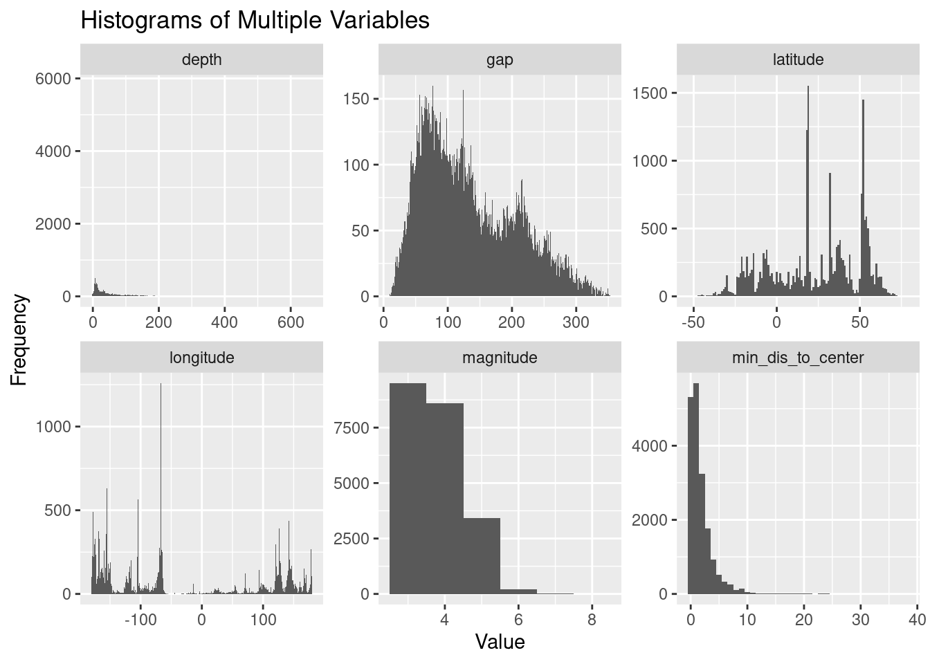
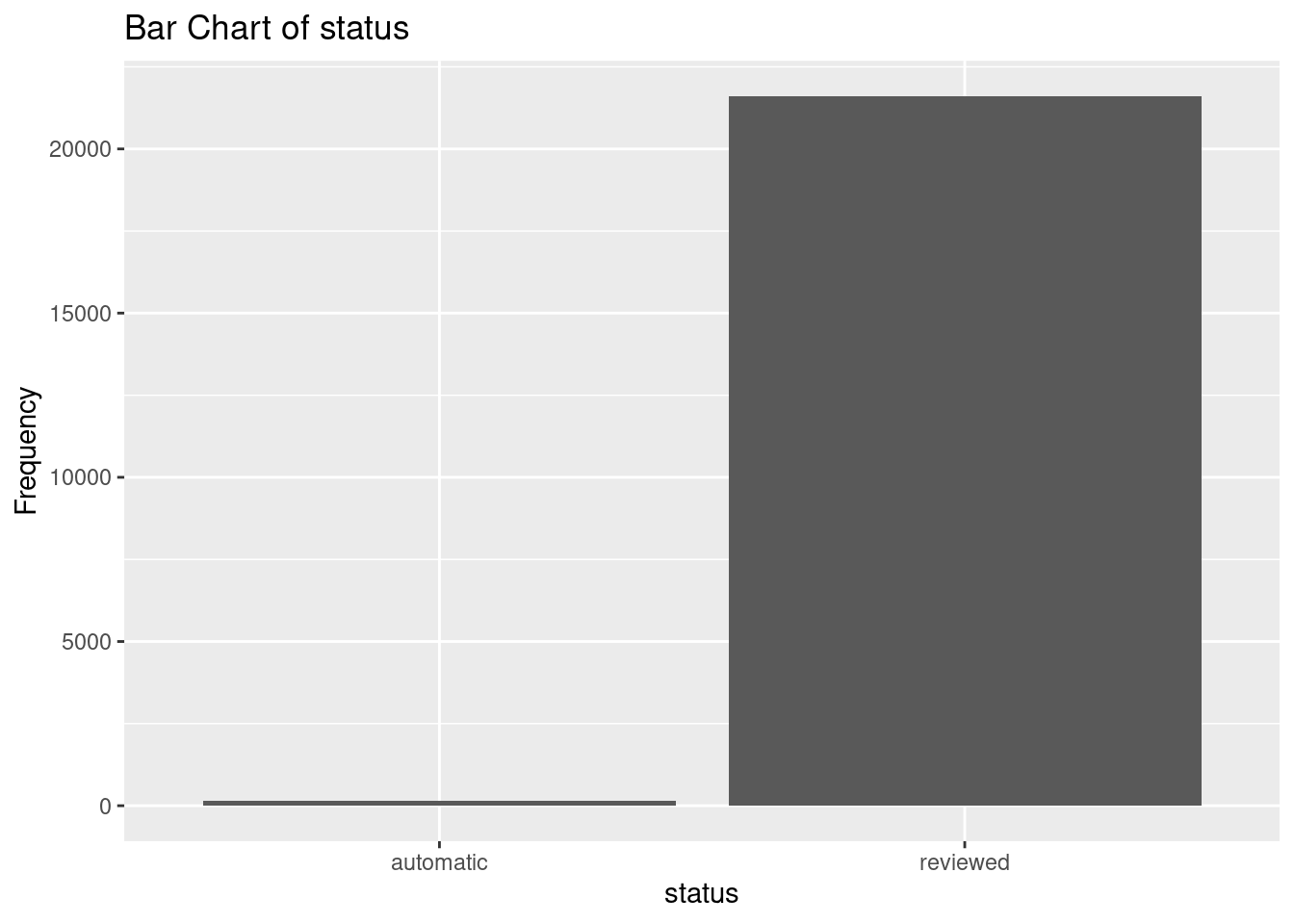
# Create and display bar charts for each categorical variable
earthquakes_cat <- earthquakes |>
  select(
    month,
    source,
    country,
    status
  )
for (var in names(earthquakes_cat)) {
  p <- ggplot(earthquakes_cat, aes(x = .data[[var]]) ) +
    geom_bar() +
    labs(title = paste("Bar Chart of", var),
         x = var,
         y = "Frequency")

  print(p)
}
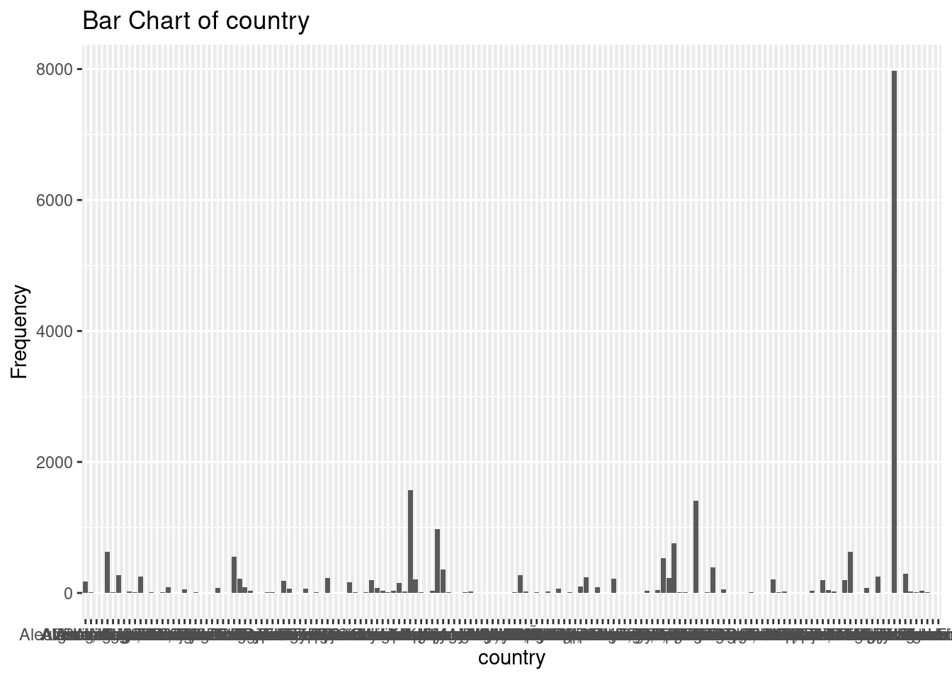
earthquakes |>
  group_by(country) |>
  summarise(
    count = n()
  ) |>
  arrange(desc(count)) |>
  head(3)
# A tibble: 3 × 2
country count
<chr> <int>
1 United States 7972
2 Indonesia 1569
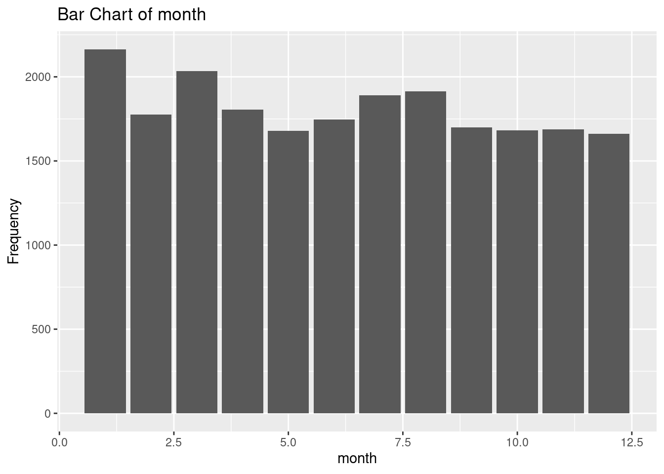
3 Puerto Rico 1412- Month: the distribution for this variable is right skewed. More earthquakes are reported in the later months in the year of 2022-2023.
- Latitude: the distribution is negative-skewed. However, most of the earthquakes reported at positive latitudes, which are located the the north of the equator. Most of them occurred at ~20 degree and ~50 degree.
- Longitude: the distribution is bi-modal. Most of the earthquakes reported at negative longitudes; in other words, a particular earthquakes occurred in the western hemisphere more often. Almost no earthquakes reported at the prime meridian. It has a standard deviation of 127 degree, which the events/data point are very diverse and spread out. The data cover a wide geographic area.
- magnitude: the reported earthquakes have an average of 3.85 and a median of 4.2, which these consider as moderate or light earthquakes. Within 2022-2023, the minimum magnitude being reported is 2.5 and the reported maximum is 7.8.
- gap: the earthquake gap distribution is bi-modal, right-skewed. Azimuuthal gap of ~100 and ~200 are the two most frequent range of reported earthquakes. On average, a reported event has an Azimuuthal gap of 128.3 degree. A standard deviation of 7.04 in azimuthal gap values suggests that the reliability of calculated horizontal earthquake positions varies. Larger values of azimuthal gap indicate less reliable or more uncertain earthquake locations.
- min_dis_to_center: the minimum horizontal distance from the epicenter to the nearest station range from 0 to 52 degrees. The median value is 1.3 and average is 2.6 degree. Most of the earthquakes are very reliable given these values are small.
- depth: the depth of reported earthquakes ranged from -3.74 to 681.2 km. It has a median of 18.8 and an average of 64.4. Data points are highly variate, with a standard deviation of 114 km.
months: most earthquakes are reported in September October
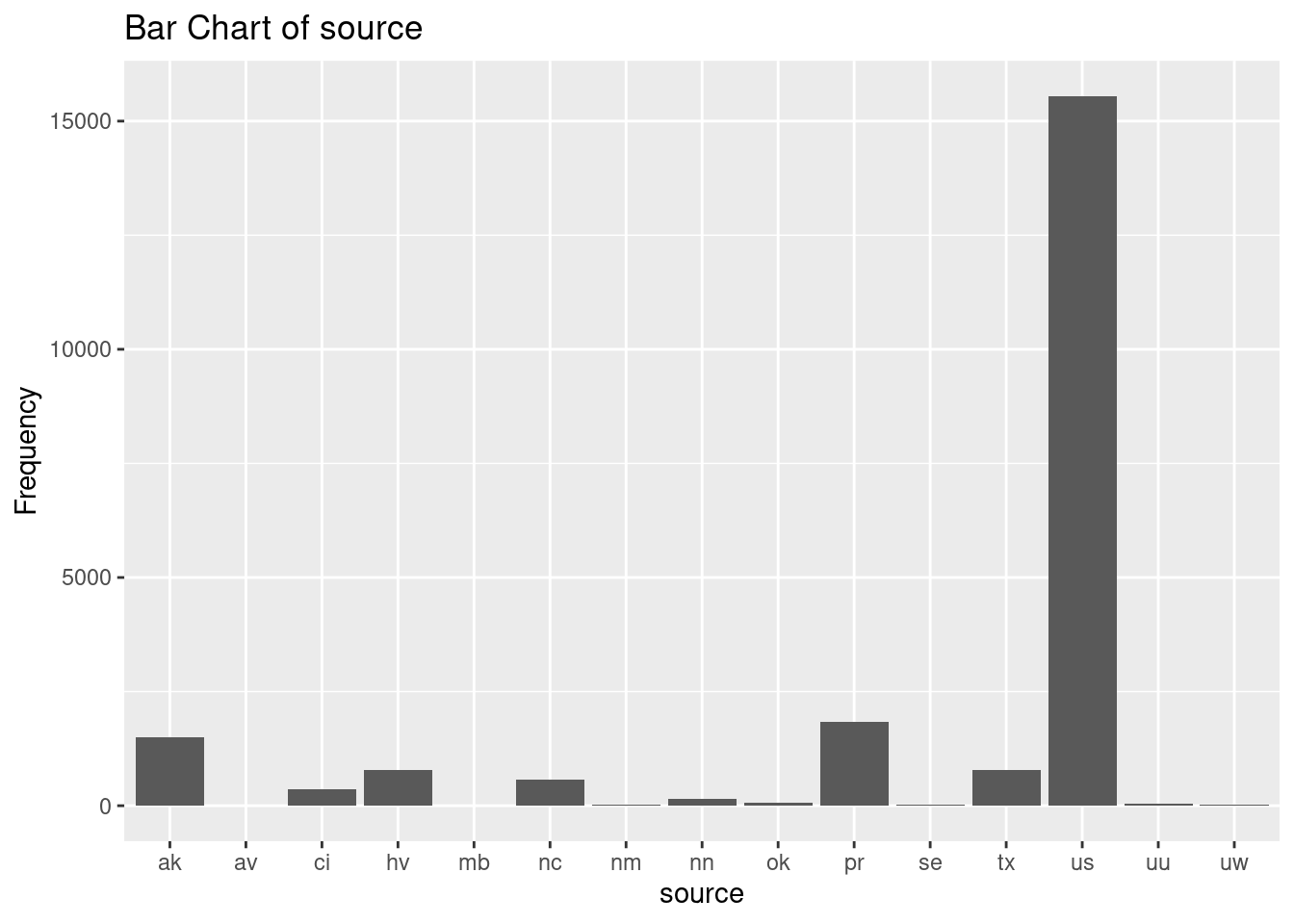
Sources: most events are sourced from the US.
Country: United States, Indonesia, and Puerto Rico are the top three countries that has the most earthquake reported within the selected timeframe.
Data limitations
Incomplete Data Coverage: Data value might not be inaccurate and might be missing due to technology limitation. For instance, the magnitude might be inaccurate (overestimated/underestimated) when the earthquake location is too far from to the The position uncertainty of the hypocenter location varies from about 100 m horizontally and 300 meters vertically for the best located events, those in the middle of densely spaced seismograph networks, to 10s of kilometers for global events in many parts of the world. Therefore, any
Variability in monitoring equipment: Differences in the quality and sensitivity of seismic networks and data collection, determination methods can affect the accuracy and consistency of earthquake data.
Data Manipulation or Exclusions: Data may be manipulated, censored, or selectively reported for various reasons, including political, economic, or security concerns, which can impact the accuracy of the available data.
Data Privacy and Security: Privacy and security concerns may limit access to certain earthquake data, especially in sensitive or classified areas.
Exploratory data analysis
Analysis 1: What is the geometric distribution of earthquakes?
library(ggplot2)

earthquakes |>
  ggplot(aes(x=longitude, y=latitude)) +
    geom_point(aes(color = magnitude),
               alpha=0.1) +
  scale_x_continuous(labels = function(breaks) paste0(breaks, "°")) +
  scale_y_continuous(labels = function(breaks) paste0(breaks, "°")) +
    labs(
      title="Geometric distribution of earthquakes",
      x="Longitude",
      y="Latitude"
    )  + theme_minimal()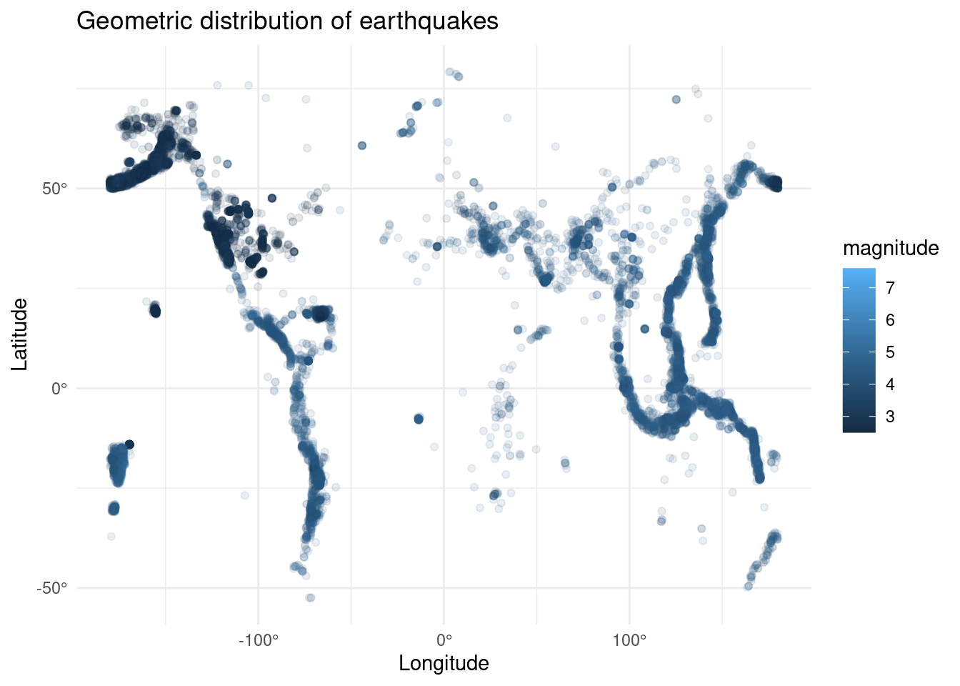
Analysis 2: What is the magnitudes distribution pattern of earthquakes in 2022 and 2023?
earthquakes |>
  ggplot(aes(x=magnitude)) +
    geom_histogram(bins=30) +
    labs(
      title="Magnitudes Distribution of Earthquake in 2022 and 2023",
      x="Magnitude",
      y="Frequency"
      ) + theme_minimal() + facet_wrap(~year) +
  scale_y_log10()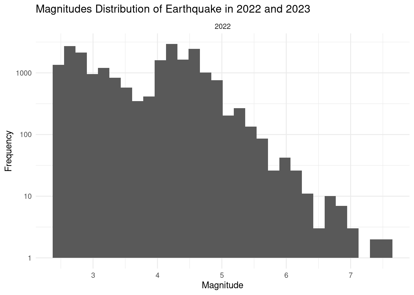
Analysis 3: What is the monthly distribution of earthquakes in 2022 and 2023?
earthquakes |>
  ggplot(aes(x=month, fill = month)) +
    geom_bar(show.legend = FALSE) +
    labs(
      title="Monthly Distribution of Earthquake Frequency",
      x="Month",
      y="Frequency"
      ) + theme_minimal() + facet_wrap(~year)
Warning: The following aesthetics were dropped during statistical transformation: fill
ℹ This can happen when ggplot fails to infer the correct grouping structure in
the data.
ℹ Did you forget to specify a `group` aesthetic or to convert a numerical
variable into a factor?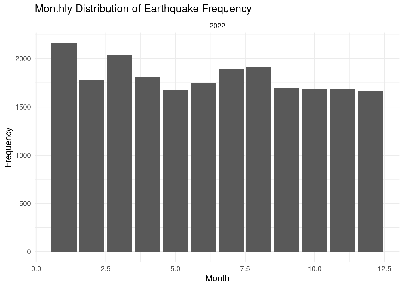
Analysis 4: Which places have the highest magnitude earthquakes?
top_locations <- earthquakes |>
                  group_by(country) |>
                  summarise(max_magnitude = max(magnitude)) |>
                  arrange(-max_magnitude) |>
                  head(10)

top_locations |>
  ggplot(aes(x=reorder(country, -max_magnitude),
             y=max_magnitude, fill=country)) +
    geom_bar(stat="identity", show.legend = FALSE) +
    labs(
      title="Top 10 Locations with Highest Magnitude Earthquakes",
      x="Location", y="Magnitude") +
    theme_minimal() +
    theme(axis.text.x = element_text(angle = 45, hjust = 1))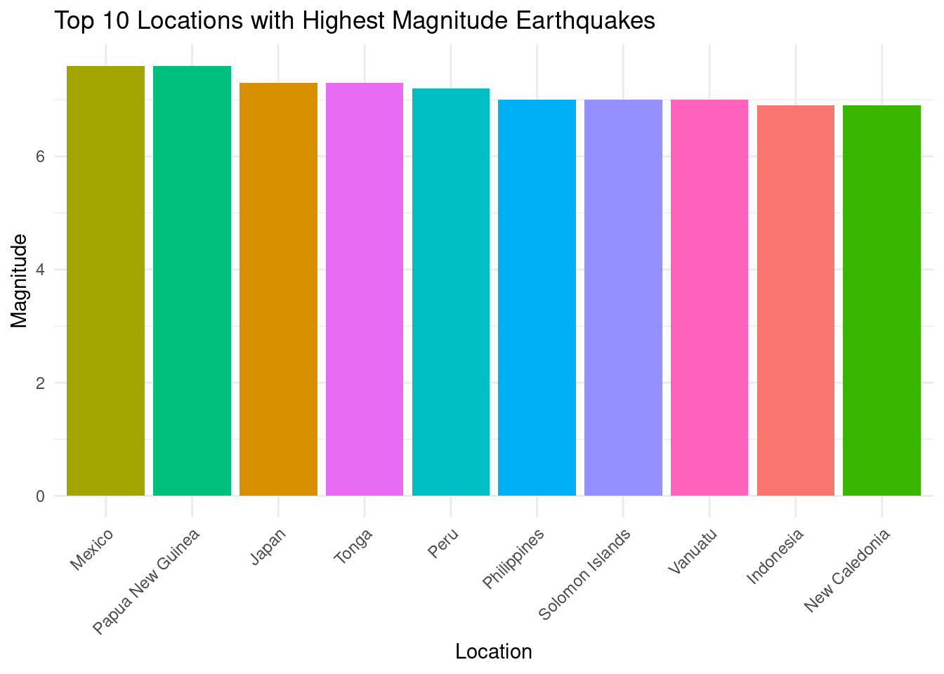
rm(top_locations)Analysis 5: Summary Stats
earthquakes |>
  summarize(
    min(min_dis_to_center),
    mean(depth),
    mean(magnitude)
  )
# A tibble: 1 × 3
`min(min_dis_to_center)` `mean(depth)` `mean(magnitude)`
<dbl> <dbl> <dbl>
1 NA 54.2 3.74Questions for reviewers
- When exploring the location of earthquakes, we want to create 2 maps: a world-map and a US map. However, we don’t want to have duplicate functionalities or interactions so still unsure how to make each of them stand out and present different information to the audience.
- Some attributes are collected using different methods/algorithm. How shall we reduce the variance resulted from these different data collection method?